$B_{s}$ mesons from the lattice: Excited states

Abstract

The energies of different angular momentum states of a heavy-light meson were measured on a lattice in [1]. We have now continued this study using several different lattices, quenched and unquenched, that have different physical lattice sizes, clover coefficients, hopping parameters and quark–gluon couplings. The heavy quark is taken to be infinitely heavy, whereas the light quark mass is approximately that of the strange quark. By interpolating in the heavy and light quark masses we can thus compare the lattice results with the $B_{s}$ meson. Most interesting is the lowest P-wave $B_{s}$ state, since it is possible that it lies below the $BK$ threshold and hence is very narrow. Unfortunately, there are no experimental results on P-wave $B_{s}$ mesons available at present.

In addition to the energy spectrum, we measured earlier also vector (charge) and scalar (matter) radial distributions of the light quark in the S-wave states of a heavy-light meson on a lattice [2]. Now we are extending the study of radial distributions to P-wave states.

1 Energies

For simplicity we consider a system that consists of one infinitely heavy quark (or anti-quark) and one light anti-quark (quark). The basic quantity for evaluating the energies of this heavy-light system on a lattice is the 2-point correlation function $C_{2}$ — see Fig. 1 a). It is defined as

$$C_{2}(T)=\langle P_{t}\Gamma G_{q}(\mathbf{x},t+T,t)\\ \cdot P_{t+T}\Gamma^{{\dagger}}U^{Q}(\mathbf{x},t,t+T)\rangle,$$ (1)

where $U^{Q}$ is the heavy quark propagator and $G_{q}$ the light anti-quark propagator. $P_{t}$ is a linear combination of products of gauge links at time $t$ along paths $P$ and $\Gamma$ defines the spin structure of the operator. The $\langle...\rangle$ means the average over the whole lattice. The energies are then extracted by fitting the $C_{2}$ with a sum of exponentials,

$$C_{2}(T)\approx\sum_{i=1}^{N_{\textrm{max}}}c_{i}\mathrm{e}^{-m_{i}T},$$ (2)

where the number of exponentials, $N_{\textrm{max}}$, is 2, 3, or 4 and the time range $T\leq 10$. $C_{2}(T)$ is in practice a $3\times 3$ matrix for different fuzzings (the indices are omitted in Eq. 2 for clarity). This fuzzing enables us to extract not only a more accurate value of $m_{1}$, the energy of the ground state, but also an estimate of the first radially excited state, $m_{2}$. After taking the continuum limit we can interpolate in the light quark mass and use charmed meson experimental results to interpolate in the heavy quark mass to get a $B_{s}$ meson. The energy spectrum was measured using different lattices: Q3 is a $16^{3}\times 24$ quenched lattice (for more details see [1]), DF2 is a $16^{3}\times 24$ lattice and DF3, DF4 are $16^{3}\times 32$ unquenched lattices. DF refers to dynamical fermions (more details can be found in [3]). Parameters of the lattices are given in Table 1.

Table 1: Lattice parameters. Here Q means quenched and DF means unquenched (dynamical fermions).

	$\beta$	$C_{\textrm{SW}}$	$\kappa$
Q3	5.7	1.57	0.14077
DF2	5.2	1.76	0.1395
DF3	5.2	2.0171	0.1350
DF4	5.2	2.0171	0.1355
	$a$ [fm]	$m_{q}/m_{s}$	$r_{0}m_{\pi}$
Q3	0.179(9)	0.83	1.555(6)
DF2	0.152(8)	1.28	1.94(3)
DF3	0.110(6)	1.12	1.93(3)
DF4	0.104(5)	0.57	1.48(3)

Figure 1: a) Two-point correlation function $C_{2}$; b) Three-point correlation function $C_{3}$.

a)	b)

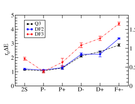
Figure 2: The energy spectrum for different angular momentum states. The notation is explained in the text. 2S is the first radially excited $L=0$ state. Here $r_{0}=0.525(25)$ fm.

From some theoretical considerations [4] it is expected that, for higher angular momentum states, the multiplets should be inverted compared with the Coulomb spectrum. If the potential is purely of the form $1/r$ the state L$+$ lies always higher than L$-$. Here L$+$($-$) means that the light quark spin couples to orbital angular momentum L giving the total $j=L\pm 1/2$. (Since the heavy quark is infinitely heavy its spin does not play a role here.) However, in the case of QCD the confining potential is important for large distances and thus L$-$ should eventually lie higher than L$+$ for higher angular momentum states. Experimentally this inversion is not seen for P-waves, and now the lattice measurements show that there is no inversion in the D-wave states either. In fact, the D$+$ and D$-$ states seem to be nearly degenerate, i.e. the spin-orbit splitting is very small (see Fig. 2). Note that the spectrum in Fig. 2 shows an approximately linear rise in excitation energy with L.

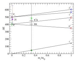
Figure 3: Interpolation from infinite mass to $m_{Q}=m_{b}$. The results at $m_{Q}=m_{c}$ are from charmed meson experiments. Note that the lowest $B_{s}$ P-wave state ($0^{+}$) lies below the $BK$ threshold and should be very narrow.

2 Radial distributions

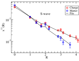
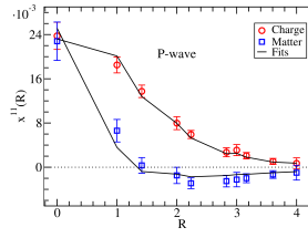
Figure 4: Ground state vector and scalar radial distributions and discretized exponential fits.

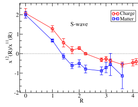
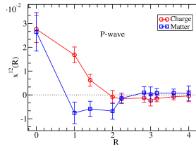
Figure 5: Radial distributions containing the first radially excited state (Ref. [2] for the S-wave).

For evaluating the radial distributions of the light quark a three-point correlation function is needed — see Fig. 1 b). It is defined as

$$C_{3}(R,T)=\langle\Gamma^{{\dagger}}U^{Q}\Gamma G_{q1}\Theta G_{q2}\rangle.$$ (3)

We have now two light anti-quark propagators, $G_{q1}$ and $G_{q2}$, and a probe $\Theta(R)$ at distance $R$ from the static quark. We have used two probes: $\gamma$₄ for the vector (charge) and $\mathbf{1}$ for the scalar (matter) distribution. The radial distributions, $x^{ij}(R)$’s, are then extracted by fitting the $C_{3}$ with

$$C_{3}(R,T)\approx\sum_{i,j=1}^{N_{\textrm{max}}}c_{i}\mathrm{e}^{-m_{i}t_{1}}x^{ij}(R)\mathrm{e}^{-m_{j}t_{2}}c_{j}$$ (4)

— see Figs. 4, 5. The $m_{i}$’s and $c_{i}$’s are from the best fit to $C_{2}$ (Eq. 2). Here $x^{11}$ is the ground state distribution and $x^{12}$, for example, is the overlap between the ground state and the first excited state.

Fig. 4 compares the ground state vector (charge) distribution with the scalar (matter) distribution. The matter distribution seems to drop off faster than the charge distribution. However, at $R=0$ the charge and matter distributions are roughly equal. Also note that the P-wave matter distribution changes its sign. (Hence the logarithmic scale in the S-wave plot but a linear scale in the P-wave plot in Fig. 4.) In Fig. 5 the charge and matter first excited state distributions are compared. As expected, a node is clearly seen in these excited state distributions. The radial distributions shown here are for DF2, but the analogous calculations for DF3 and DF4 are in progress. These distributions can be now treated as “experimental data” that needs understanding.

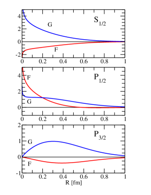
Figure 6: Dirac equation numerical solutions, F and G, for a potential $V=-e/R+b\cdot R$. Here $e=0.6\cdot\hslash c$, $b=(500~{}\textrm{MeV})^{2}$ and $m=100$ MeV.

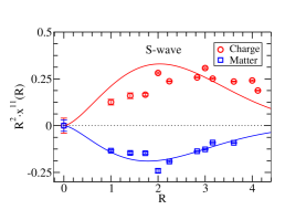
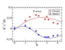
Figure 7: Dirac equation numerical solutions for the same potential as in Figure 6 compared with lattice results. $R$ is given in lattice units ($a\approx 0.15$ fm). Here the sign of the S-wave matter distribution has been changed for clarity.

The lattice measurements, i.e. the energy spectrum and the radial distributions, can be used to test potential models. There are several advantages for model makers: First of all, since the heavy quark is infinitely heavy, we have essentially a one-body problem. Secondly, on the lattice we know what we put in — one heavy quark and one light anti-quark — which makes the lattice system much more simple than the real world. We can, for example, try to use the Dirac equation to interpret the S- and P-wave distributions. If the solutions of the Dirac equation are called $G$ (the “large” component) and $F$ (the “small” component) we get

$$x^{11}(R)=G(R)^{2}+F(R)^{2}$$ (5)

for the charge distribution and

$$x^{11}(R)=G(R)^{2}-F(R)^{2}$$ (6)

for the matter distribution. These solutions are plotted in Fig. 6 for a potential $V=-e/R+b\cdot R$, where $e=0.6\cdot\hslash c$, $b=(500~{}\textrm{MeV})^{2}$ and the mass that appears in the Dirac equation is $m=100$ MeV. The values of these parameters are not tuned yet, because at this stage we only want to show that a reasonable set of parameters can give a qualitative description of the lattice data. The qualitative agreement is surprisingly good — see Fig. 7. The Dirac equation approach gives a natural explanation, for example, to the fact that the matter distribution drops off faster than the charge distribution. Also the change of sign in the P-wave matter distribution comes out automatically.

3 Main conclusions

The key points are:

• There should be several narrow $B_{s}$ states, in particular the $0^{+}$ that lies below the $BK$ threshold.

• The spin-orbit splitting is very small, contrary to the expectation predicted by a linearly rising potential that is purely scalar.

• The radial distributions of S and P$-$ states can be qualitatively understood by using a Dirac equation model.

The natural next step would be to calculate the radial distributions for P$+$, D$-$, D$+$ and F-wave states.

References

- [1] C. Michael and J. Peisa for UKQCD Collaboration, Phys. Rev. D 58, 34506 (1998), hep-lat/9802015.
- [2] A.M. Green, J. Koponen, C. Michael and P. Pennanen for UKQCD Collaboration, Phys. Rev. D 65, 014512 (2002) and Eur. Phys. J. C 28, 79 (2003), hep-lat/0206015
- [3] A.M. Green, J. Koponen, C. McNeile, C. Michael and G. Thompson for UKQCD Collaboration, Phys. Rev. D 69, 094505 (2004), hep-lat/0312007.
- [4] H. J. Schnitzer, Phys. Rev. D 18, 3482 (1978) and Phys. Lett. B 226, 171 (1989).