Instantons and Monte Carlo Methods in Quantum Mechanics

Abstract

In these lectures we describe the use of Monte Carlo simulations in understanding the role of tunneling events, instantons, in a quantum mechanical toy model. We study, in particular, a variety of methods that have been used in the QCD context, such as Monte Carlo simulations of the partition function, cooling and heating, the random and interacting instanton liquid model, and numerical simulations of non-Gaussian corrections to the semi-classical approximation.

I Introduction

We consider a non-relativistic particle moving in a potential $V(x)$. The Hamiltonian of the system is given by

$$H=\frac{p^{2}}{2m}+\lambda\left(x^{2}-\eta^{2}\right)^{2}.$$ (1)

We can rescale $x$ and $t$ such that $2m=\lambda=1$. We will also use $\hbar=1$. This means that the system is characterized by just one dimensionless parameter, $\eta$. The potential $V(x)$ with $\eta=1.4$ is shown in Fig. 1a. The physics of this system is easy to understand. Classically, there are two degenerate minima at $x=\pm\eta$. Quantum mechanically, the two states can mix. If the potential barrier is very high, $\eta\to\infty$, the wave functions of the ground state and the first excited state are approximately given by

$$\psi_{0,1}(x)=\frac{1}{\sqrt{2}}(\psi_{-}(x)\pm\psi_{+}(x)),$$ (2)

where $\psi_{\pm}(x)$ are the ground state wave functions in the left and right minimum of the potential. The energy splitting between the ground state and the first excited state is exponentially small. The WKB approximation gives

$$\Delta E=E_{1}-E_{0}=\sqrt{\frac{6S_{0}}{\pi}}\omega\exp(-S_{0}),$$ (3)

where $\omega=4\eta$ and $S_{0}=m^{2}\omega^{3}/(12\lambda)=4\eta^{3}/3$.

Applications of the WKB method and of instantons to the double well potential are discussed in many reviews and text books Polyakov:1976fu ; Vainshtein:1981wh ; Coleman:1978ae ; Shuryak:1988ck ; Kleinert:1995 ; Zinn-Justin:1993wc ; Schafer:1996wv ; Forkel:2000sq . It is not our intention to present another review on the subject in these lecture notes. Instead, we will use the double well potential to illustrate a number of numerical methods that have proven useful in the context of QCD and other gauge theories.

II Exact Diagonalization

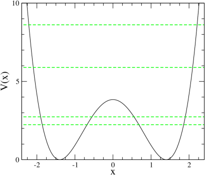
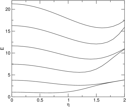
Figure 1: a) Double well potential $V(x)=(x^{2}-\eta^{2})^{2}$ for $\eta=1.4$. We have indicated the position of the ground state and the first three excited state. b) Spectrum of the double well potential as a function of the parameter $\eta$. In this figure we show the position of the first six states. We clearly observe that positive and negative parity states become degenerate as $\eta\to\infty$.

The quantum mechanical problem defined by the Hamiltonian equ. (1) can be solved by determining the eigenvalues and eigenvectors of $H$. This can be achieved by choosing a basis and numerically diagonalizing the Hamilton operator in that basis. We have chosen a simple harmonic oscillator basis defined by the eigenstates of

$$H_{0}=\frac{p^{2}}{2m}+\frac{1}{2}m\omega_{0}^{2}x^{2}.$$ (4)

The value of $\omega_{0}$ is arbitrary, but the truncation error of the eigenvalues computed in a finite basis will depend on the choice of $\omega_{0}$. In practice, however, this dependence is quite weak. The eigenstates of $H_{0}$ satisfy $H_{0}|n\rangle=|n\rangle\omega_{0}(n+1/2)$. The Hamiltonian of the anharmonic oscillator has a very simple structure in this basis. The only non-zero matrix elements are

$$\langle n|H|n\rangle = 3Ac^{4}\left[(n+1)^{2}+n^{2}\right]+Bc^{2}(2n+1)+\omega_{0}(n+1/2)+c,$$ (5)

$$\langle n|H|n+2\rangle = Ac^{4}(4n+6)\sqrt{(n+1)(n+2)}+Bc^{2}\sqrt{(n+1)(n+2)},$$ (6)

$$\langle n|H|n+4\rangle = c^{4}\sqrt{(n+1)(n+2)(n+3)(n+4)},$$ (7)

as well as the corresponding hermitian conjugates. We have also defined $A=1$, $B=-2\eta^{2}-\omega_{0}^{2}/4$, $C=\eta^{4}$ and $c=1/\sqrt{\omega_{0}}$. Note that both $H$ and $H_{0}$ conserve parity. We can decompose the matrix $H_{nm}=\langle n|H|m\rangle$ into even and odd components, $H=H_{even}+H_{odd}$, such that the eigenvectors of $H_{even}$ and $H_{odd}$ have positive and negative parity, respectively.

With the choice $\omega_{0}=4\eta$ even modest basis sizes such as $N=40$ are sufficient in order to determine the first few eigenvectors very accurately. In Fig. 1b we show the first six eigenvalues as a function of the parameter $\eta$. We clearly observe that as $\eta$ increases pairs of eigenvalues corresponding to even and odd eigenfunctions become almost degenerate. In this limit the eigenfunctions are of the form given in equ. (2).

III Quantum Mechanics on a Euclidean Lattice

An alternative to the Hamiltonian formulation of the problem is the Feynman path integral Feynman . The path integral for the anharmonic oscillator is given by

$$\langle x_{1}|e^{-iHt_{1}}|x_{0}\rangle=\int_{x(0)=x_{0}}^{x(t_{1})=x_{1}}{\cal D}x\,e^{iS},\hskip 28.45274ptS=\int_{0}^{t_{1}}dt\,\left(\frac{1}{4}\dot{x}^{4}-(x^{2}-\eta^{2})^{2}\right).$$ (8)

In the following we shall consider the euclidean partition function

$$Z(T)=\int{\cal D}x\,e^{-S_{E}},\hskip 28.45274ptS_{E}=\int_{0}^{\beta}d\tau\,\left(\frac{1}{4}\dot{x}^{4}+(x^{2}-\eta^{2})^{2}\right),$$ (9)

where $\beta=1/T$ is the inverse temperature. The partition function can be expressed in terms of the eigenvalues of the Hamiltonian, $Z(T)=\sum_{n}\exp(-E_{n}/T)$. In the following we shall study numerical simulations using a discretized euclidean action. For this purpose we discretize the euclidean time coordinate $\tau_{i}=ia,\,i=1,\ldots n$. The discretized action is given by

$$S=\sum_{i=1}^{n}\left\{\frac{1}{4a}(x_{i}-x_{i-1})^{2}+a(x_{i}^{2}-\eta^{2})^{2}\right\},$$ (10)

where $x_{i}=x(\tau_{i})$. We shall consider periodic boundary conditions $x_{0}=x_{n}$. The discretized euclidean path integral is formally equivalent to the partition function of a statistical system of “spins” $x_{i}$ arranged on a one-dimensional lattice. This statistical system can be studied using standard Monte-Carlo sampling methods. In the following we will simply use the Metropolis algorithm Creutz:1980gp ; Shuryak:1984xr ; Shuryak:1987tr . The Metropolis method generates an ensemble of configurations $\{x_{i}\}^{(k)}$ where $i=1,\ldots,n$ labels the lattice points and $k=1,\ldots,N_{conf}$ labels the configurations. Quantum mechanical averages are computed by averaging observables over many configurations,

$$\langle{\cal O}\rangle=\lim_{N_{conf}\to\infty}\frac{1}{N_{conf}}\sum_{k=1}^{N_{conf}}{\cal O}^{(k)}$$ (11)

where ${\cal O}^{(k)}$ is the value of the classical observable ${\cal O}$ in the configuration $\{x_{i}\}^{(k)}$. The configurations are generated using Metropolis updates $\{x_{i}\}^{(k)}\to\{x_{i}\}^{(k+1)}$. The update consists of a sweep through the lattice during which a trial update $x_{i}^{(k+1)}=x_{i}^{(k)}+\delta x$ is performed for every lattice site. Here, $\delta x$ is a random number. The trial update is accepted with probability

$$P\left(x_{i}^{(k)}\to x_{i}^{(k+1)}\right)=\min\left\{\exp(-\Delta S),1\right\},$$ (12)

where $\Delta S$ is the change in the action equ. (10). This ensures that the configurations $\{x_{i}\}^{(k)}$ are distributed according the “Boltzmann” distribution $\exp(-S)$. The distribution of $\delta x$ is arbitrary as long as the trial update is micro-reversible, i. e. is equally likely to change $x_{i}^{(k)}$ to $x_{i}^{(k+1)}$ and back. The initial configuration is also arbitrary. In order to study equilibration it is often useful to compare an ordered (cold) start with $\{x_{i}\}^{(0)}=\{\eta\}$ to a disordered (hot) start $\{x_{i}\}^{(0)}=\{r_{i}\}$, where $r_{i}$ is a random variable.

The advantage of the Metropolis algorithm is its simplicity and robustness. The only parameter to adjust is the distribution of $\delta x$. We typically take $\delta x$ to be a Gaussian random number with the width of the distribution adjusted such that the average acceptance rate for the trial updates is around $50\%$. Fluctuations of ${\cal O}$ provide an estimate in the error of $\langle{\cal O}\rangle$. We have

$$\Delta\langle{\cal O}\rangle=\sqrt{\frac{\langle{\cal O}^{2}\rangle-\langle{\cal O}\rangle^{2}}{N_{conf}}}.$$ (13)

This requires some care, because the error estimate is based on the assumption that the configurations are statistically independent. In practice this can be monitored by computing the auto-correlation “time” in successive measurements ${\cal O}(\{x_{i}\}^{(k)})$. The auto-correlation time of different observables can be very different. For example, successive measurements of the total energy decorrelate very quickly, but measurements of the topological charge have a much longer correlation time.

The energy eigenvalues and wave functions of the quantum mechanical problem can be obtained from the euclidean correlation functions

$$\Pi(\tau)=\langle O(0)O(\tau)\rangle.$$ (14)

Here, $O(\tau)$ is an operator that can be constructed from the variables $x(\tau)$, e.g. some integer power $O(\tau)=x(\tau)^{n}$. The euclidean correlation functions are related to the quantum mechanical states via spectral representations. The spectral representation is obtained by inserting a complete set of states into the expectation value equ. (14). We find

$$\Pi(\tau)=\sum_{n}|\langle 0|O(0)|n\rangle|^{2}\exp(-(E_{n}-E_{0})\tau),$$ (15)

where $E_{n}$ is the energy of the state $|n\rangle$ and $|0\rangle$ is the ground state of the system. We can write this as

$$\Pi(\tau)=\int dE\,\rho(E)\exp(-(E-E_{0})\tau).$$ (16)

In the case we are studying here there are only bound states and the spectral function $\rho(E)$ is a sum of delta-functions. Equ. (15) shows that the euclidean correlation function is easy to construct once the energy eigenvalues and eigenfunctions are known. This fact was used in order to calculate the solid lines shown in Figs. (4). The inverse problem is well defined in principle, but numerically much harder. In the following we will concentrate on extracting just the first few energy levels. A technique that can be used on order determine the spectral function from euclidean correlation functions is the maximum entropy image reconstruction method, see Jarrel:1996 ; Asakawa:2000tr .

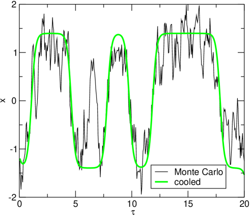
Figure 2: Typical euclidean path obtained in a Monte Carlo simulation of the discretized euclidean action of the double well potential for $\eta=1.4$. The lattice spacing in the euclidean time direction is $a=0.05$ and the total number of lattice points is $N_{\tau}=800$. The green curve shows the corresponding smooth path obtained by running 100 cooling sweeps on the original path.

The Monte Carlo method is very useful in calculating expectation values in quantum or statistical mechanics. However, the Monte Carlo method does not directly give the partition function or the free energy. In principle one can reconstruct the free energy from the energy eigenvalues but this is not very practical since, as we just mentioned, it is hard to compute the full spectrum. A very effective method for computing the free energy is the adiabatic switching technique. The idea is to start from a reference system for which the free energy is known and calculate the free energy difference to the real system using Monte Carlo methods.

For this purpose we write the action as $S_{\alpha}=S_{0}+\alpha\Delta S$ where $S$ is the full action, $S_{0}$ is the action of the reference system, $\Delta S$ is defined by $\Delta S=S-S_{0}$, and $\alpha$ is a coupling constant. The action $S_{\alpha}$ interpolates between the real and the reference system. Integrating the relation $\partial\log Z(\alpha)/(\partial\alpha)=-\langle\Delta S\rangle_{\alpha}$ we find

$$\log(Z(\alpha=1))=\log(Z(\alpha=0))-\int_{0}^{1}d\alpha^{\prime}\,\langle\Delta S\rangle_{\alpha^{\prime}}\;\;,$$ (17)

where $\langle.\rangle_{\alpha}$ is an expectation value calculated using the action $S_{\alpha}$. In the present case it is natural to use the harmonic oscillator as a reference system. In that case

$$Z(\alpha=0)=\sum_{n}\exp(-\beta E_{n}^{0})=\frac{\exp(-\beta\omega_{0}/2)}{1-\exp(-\beta\omega_{0})},$$ (18)

where $\omega_{0}$ is the oscillator constant. Note that the free energy of the anharmonic oscillator should be independent of $\omega_{0}$. The integral over the coupling constant $\alpha$ can easily be calculated in Monte Carlo simulations by slowly changing $\alpha$ from 0 to 1 during the simulation. In order to estimate systematic errors due to incomplete equilibration it is useful to repeat the calculation with $\alpha$ changing from 1 to 0 and study possible hysteresis effects.

IV Numerical Results

Numerical results from Monte Carlo simulations of the euclidean path integral are shown in Figs. 2-4. The numerical data were obtained using the program qm.for which is described in more detail in the appendix. A typical path that appears in the Monte Carlo simulation is shown in Fig. 2. The figure clearly shows that there are two characteristic time scales in the problem. On short time scales the motion is controlled by the oscillation time $\tau_{osc}\sim\omega^{-1}\sim(4\eta)^{-1}$. For large $\tau$ the system is governed by the tunneling time $\tau_{tun}\sim\exp(-4\eta^{3}/3)$. In order to perform reliable simulations we have to make sure that the lattice spacing $a$ is small compared to $\tau_{osc}$ and that the total length of the lattice $Na$ is much larger than the tunneling time

$$a\ll\tau_{osc},\hskip 14.22636pt\tau_{tun}\ll Na.$$ (19)

A typical choice of parameters for the case $\eta=1.4$ is a number of lattice points $N=800$, a lattice spacing $a=0.05$ and a number of Metropolis sweeps $N_{conf}=10^{5}$.

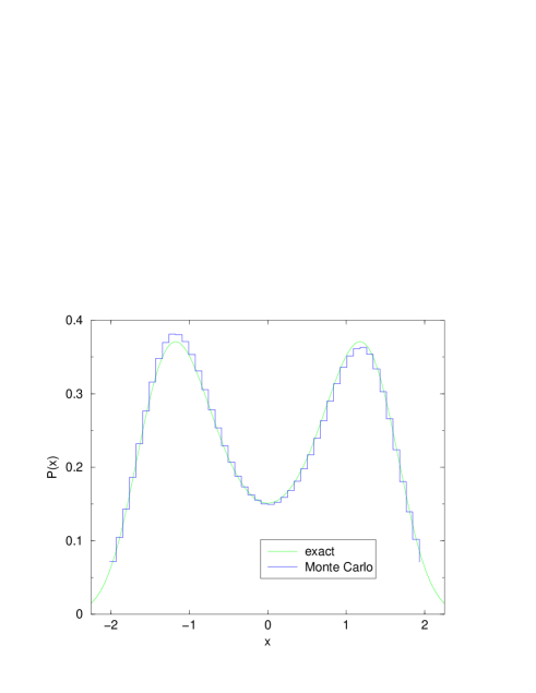
Figure 3: Probability distribution $|\psi(x)|^{2}$ in the double well potential for $\eta=1.4$. The solid line shows the “exact” numerical result obtained by diagonalizing the Hamiltonian in an oscillator basis whereas the histogram shows the distribution of $x$ for an ensemble of euclidean paths.

Fig. 3 shows the distribution of $x_{i}$ obtained in the Monte Carlo simulation compared to the square of the ground state wave function computed by the diagonalization method discussed in section II. As $\eta$ is increased and the potential barrier becomes larger the tunneling time increases exponentially and the number of configurations needed to reproduce the correct wave function becomes very large.

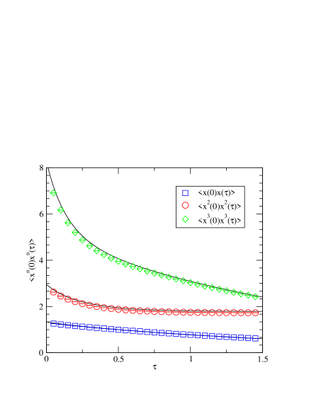
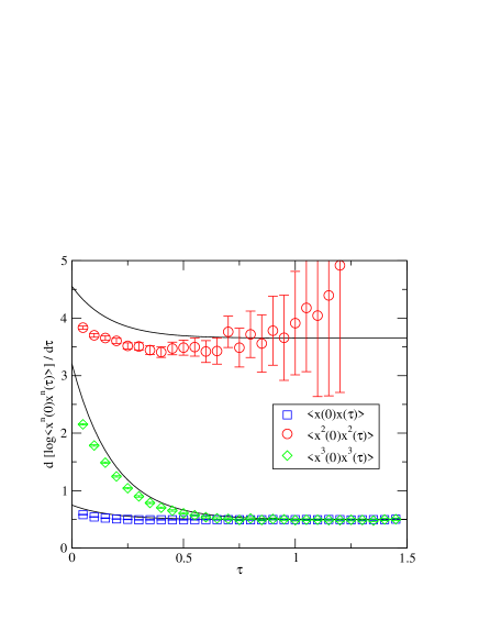
Figure 4: Fig. a shows the correlation functions $\langle{\cal O}(0){\cal O}(\tau)\rangle$ in the double well potential for $\eta=1.4$ and ${\cal O}=x,x^{2},x^{3}$. The solid lines are “exact” numerical results obtained by diagonalizing the Hamiltonian in an oscillator basis whereas the data point were obtained from Monte Carlo simulations with $a=0.05$ and $N_{\tau}=800$. Fig. b shows the logarithmic derivative of the correlators in Fig. a. In the case of the $\langle x^{2}(0)x^{2}(\tau)\rangle$ we subtracted the constant contribution.

Fig. 4 shows the correlation functions of the operators $x,x^{2}$ and $x^{3}$. The solid lines show the result obtained using the spectral representation equ. (15) together with the eigenvalues and eigenfunctions determined by numerical diagonalization of the Hamiltonian. The data points show the results from the Monte Carlo simulation. There is a small systematic disagreement for small $\tau$ which is related to discretization errors but the overall agreement is excellent. Energy levels and matrix elements can be obtained from the logarithmic derivative of the correlation function,

$$C(\tau)=-\frac{d\log\Pi(\tau)}{d\tau}=\frac{\sum_{n}(E_{n}-E_{0})|\langle 0|O(0)|n\rangle|^{2}\exp(-(E_{n}-E_{0})\tau)}{\sum_{n}|\langle 0|O(0)|n\rangle|^{2}\exp(-(E_{n}-E_{0})\tau)}.$$ (20)

In the limit $\tau\to\infty$ the function $C(\tau)$ converges to the energy splitting between the ground state and the first excited state that has a non-vanishing transition amplitude $\langle 0|O(0)|n\rangle$. Because of parity invariance, $O=x^{n}$ connects the groundstate to parity even/odd levels for $n$ even/odd. Since the first excited state is parity odd we have

$$\lim_{\tau\to\infty}\frac{d}{d\tau}\log\langle x(\tau)x(0)\rangle=\lim_{\tau\to\infty}\frac{d}{d\tau}\log\langle x^{3}(\tau)x^{3}(0)\rangle=E_{1}-E_{0}.$$ (21)

For even powers of $x$ the situation is more complicated because the correlator has a constant term $|\langle 0|x^{2n}|0\rangle|^{2}$. After subtracting the constant part, the logarithmic derivative of the correlation function of even powers of $x$ tends to $(E_{2}-E_{0})$. Numerical results are shown in Fig. 4b. We observe that the logarithmic derivative of $\langle x(\tau)x(0)\rangle$ converges very rapidly to $\Delta E_{1}=(E_{1}-E_{0})$. The numerical results for $\Delta E_{2}=(E_{2}-E_{0})$ have large uncertainties. These uncertainties are related to the fact that the correlator $\langle x^{2}(\tau)x(0)\rangle$ is dominated by the subtraction constant $\langle x^{2}\rangle^{2}$. The logarithmic derivative of the $\langle x^{3}(\tau)x^{3}(0)\rangle$ correlator also tends to $\Delta E_{1}$, but receives larger contributions from excited states. This feature can be used in order to extract the energies of higher states. The idea is very simple. From the matrix elements $c_{1}=\langle 0|x|1\rangle$ and $d_{1}=\langle 0|x^{3}|1\rangle$ we can determine a new operator ${\cal O}=x/c_{1}-x^{3}/d_{1}$ that does not couple to the first excited state. This operator predominantly couples to the third excited state. Repeating this procedure we can determine the energies of higher excited states. The problem is that correlation functions of higher powers of $x$ are more and more noisy. As a result, finding the energies of highly excited states is very hard, even in the simple problem considered here.

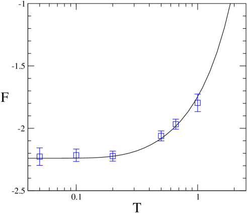
Figure 5: Free energy $F=-T\log(Z)$ of the anharmonic oscillator as a function of the temperature $T=1/\beta$ with $\beta=na$. The solid line was calculated using the spectrum of the Hamiltonian. The data points were obtained using Monte Carlo calculations and the adiabatic switching method.

In Fig. 5 we show Monte Carlo results for the partition function compared to “exact” results based on the spectrum of the anharmonic oscillator obtained in Sect. II. The Monte Carlo results agree with the direct calculations but the Monte Carlo method is effectively limited to a small range of temperatures. If the temperature is very small the partition function is dominated by the ground state contribution. In that case, it is much more efficient to compute the ground state energy directly by measuring the expectation value of the Hamiltonian, $E_{0}=\langle H\rangle$ , with $H=\dot{x}^{2}/4+V(x)$. There is one subtlety with this approach: If a naive one-sided discretization of the time derivative is used then the continuum limit of the expectation value of the kinetic energy diverges. This problem can be addressed by using an improved discretization of the kinetic energy Feynman , or by using the Virial theorem. The Virial theorem implies that

$$\langle H\rangle=\langle T+V\rangle=\langle\frac{x}{2}V^{\prime}+V\rangle.$$ (22)

At high temperature more and more states contribute. The main difficulty with the Monte Carlo approach in this regime is that discretization errors have to be carefully monitored.

V Extracting the Instanton Content using Cooling

From Fig. 2 we can clearly see that for this particular choice of the parameter $\eta$ a typical path contains two components, one related to quantum fluctuations with frequency $\omega$, and one related to tunneling events, instantons. In the continuum limit the instanton solution can be found from the classical equation of motion

$$\frac{\delta}{\delta x(\tau)}S_{E}=0\hskip 14.22636pt\Rightarrow\hskip 14.22636ptm\ddot{x}=V^{\prime}(x).$$ (23)

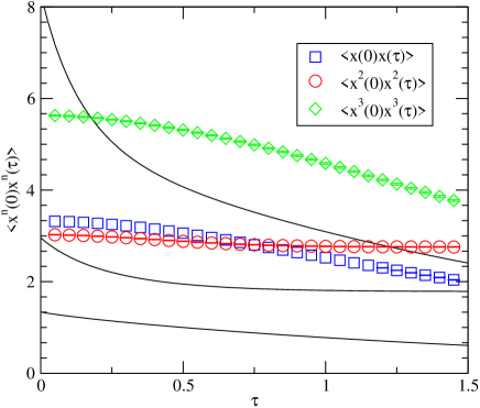
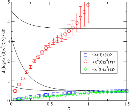
Figure 6: Same as Fig. 4 but the correlation functions are evaluated from cooled Monte Carlo configurations. The number of cooling sweeps is $N_{cool}=200$.

The solution which satisfies the boundary condition $x(\tau\to\pm\infty)=\pm\eta$ is given by

$$x_{I}(\tau)=\eta\tanh\left[\frac{\omega}{2}(\tau-\tau_{0})\right],$$ (24)

where $\omega=4\eta$ and $\tau_{0}$ is the “location” of the instanton. The anti-instanton solution is simply given by $x_{A}(\tau)=-x_{I}(\tau)$. The classical action of the instanton is

$$S_{0}=\frac{4\eta^{3}}{3}.$$ (25)

The tunneling rate $n_{I+A}=N_{I+A}/\beta$ is exponentially small, $n_{I+A}\sim\exp(-S_{0})$. In order to determine the pre-factor one has to study small fluctuations around the instanton solution. This calculation has been carried out to next-to-leading order in the semi-classical expansion. The result is Zinn-Justin:1993wc ; Kleinert:1995 ; Wohler:pg

$$n_{I+A}=8\eta^{5/2}\sqrt{\frac{2}{\pi}}\exp\left(-S_{0}-\frac{71}{72}\frac{1}{S_{0}}\right).$$ (26)

The tunneling events can be studied in more detail after removing short distance fluctuations. A well known method for doing this is “cooling” Hoek:1985gj ; Hoek:1986hq . In the cooling method we only accept Metropolis updates that lower the action. This will drive the system towards the nearest classical solution. Since instantons are classical solutions, cooling can be used to study the instanton content of a quantum configurations. This is clearly seen in Fig. 2. The black line is the original, quantum, configuration. The green line is the same configuration after 200 cooling sweeps. It is easy to check that this configuration is very close to a linear superposition of independent tunneling events. For this purpose we can extract the instanton and anti-instanton locations from the zero crossings and compare the cooled configuration to the simple “sum ansatz”

$$x_{sum}(\tau)=\eta\left\{\sum_{i}Q_{i}\tanh\left[\frac{\omega}{2}(\tau-\tau_{i})\right]-1\right\},$$ (27)

where $Q_{i}=\pm 1$ is the topological charge of the instanton. The most important question is to what extent physical observables in the cooled configurations resemble those in the original configurations. This provides a measure of the importance of instantons in the double well potential. In Fig. 6 we show correlation functions measured in the cooled configurations. These results should be compared with the full correlation functions shown in Fig. 4. We observe that the correlation functions are quite different. Short distance fluctuations eliminated by cooling obviously play an important role. We observe, however, that the level splitting between the ground state and the first excited state is clearly dominated by semi-classical configurations. The logarithmic derivative of both the $\langle x(0)x(\tau)\rangle$ and $\langle x^{3}(0)x^{3}(\tau)\rangle$ correlation functions is very well reproduced in the cooled configurations.

VI The density of instantons

The cooling method can also be used in order to get an estimate of the total density of instantons and anti-instantons. While the net topological charge, the number of instantons minus the number of anti-instantons, is unambiguously defined the same is not true for the total number of topological objects. There is no clear distinction between a large quantum fluctuation and a very close instanton-anti-instanton pair. In the cooling method this is reflected by the fact that the number of instantons, extracted from the number of zero crossings in the cooled configuration, depends on the number of cooling sweeps.

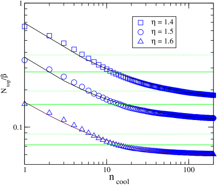
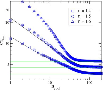
Figure 7: Instanton density and instanton action as a function of the number of cooling sweeps for different values of the parameter $\eta$. The solid and dashed green lines in Fig. a shows the semi-classical instanton density at one and two-loop order. The solid line in Fig. b shows the classical instanton action.

It is clear, however, that the instanton density should be well defined in the semi-classical limit. In this limit there is an exponentially large separation of scales between the tunneling time $\tau_{tun}$ and the scale of ordinary quantum fluctuations $\tau_{osc}$. This separation of scales can also be exploited in the cooling method. Cooling is a local algorithm which implies that it takes on the order of $\tau/a$ cooling sweeps in order to affect coherent structures that exist at a scale $\tau$. We expect that the number of instantons measured using the cooling method is approximately given by the sum of two exponentials, $N_{I}(n_{cool})=N_{osc}\exp(-n_{cool}a/\tau_{osc})+N_{tun}\exp(-n_{cool}a/\tau_{tun})$. The first exponential describes the disappearance of quantum fluctuations on a time scale $\tau_{osc}$ and the second exponential reflects instanton-anti-instanton annihilation occurring on a time scale $\tau_{tun}$.

Numerical results for $N_{I}(n_{cool})$ are shown in Fig. 7. We observe that the data is consistent with the presence of two distinct time scales and that the description in terms of two exponentials becomes better as the semi-classical limit $\eta\to\infty$ is approached. We also note that after the quantum noise has disappeared the instanton density is close to the semi-classical result equ. (26). A more detailed comparison is shown in Fig. 8. In this figure we show the instanton density after 10 cooling sweeps, the one and two-loop semi-classical result, as well as the level spacing between the ground state and the first excited state.

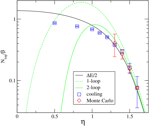
Figure 8: Instanton density as a function of the parameter $\eta$. The blue symbols show the instanton density extracted from Monte Carlo configurations after 10 cooling sweeps. The red symbols show the results of a Monte Carlo calculation of non-Gaussian effects. The green lines show the semi-classical instanton density at one and two-loop order. The black line shows $\Delta E/2$ where $\Delta E$ is the splitting between the ground state and the first excited state.

We observe that for $\eta>1.2$, corresponding to a classical instanton action $S_{0}>2$, the number of instantons extracted using the cooling method agrees very well with the semi-classical approximation. We also note that the two-loop result is a clear improvement over the one-loop approximation for classical actions as small as $S_{0}\sim 1$. Finally, we observe that the instanton density is close to the level splitting even in the regime where $S_{0}$ is less than one.

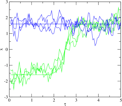
Figure 9: Quantum mechanical paths which appear in a Monte-Carlo calculation of the one-instanton partition function in the double well potential. The calculation involves adiabatic switching between the Gaussian effective potential and the full potential. The smooth curves are the initial configurations in the zero and one-instanton sector. The Monte Carlo updates in the one-instanton sector involve a constraint which keeps the instanton location fixed.

In Fig. 7 we also show a Monte Carlo calculation of the instanton density on a small lattice. The idea is very simple. The one-loop calculation of the tunneling rate is based on expanding the action around the classical path to quadratic order

$$S=S_{0}+\frac{1}{2}\int d\tau\,\delta x(\tau)\left.\frac{\delta^{2}S}{\delta x^{2}}\right|_{x_{I}(\tau)}\delta x(\tau)+\ldots,$$ (28)

where $\delta x(\tau)=x(\tau)-x_{I}(\tau)$. As in Sect. III we can introduce a new action $S_{\alpha}$ that interpolates between the full action and the Gaussian approximation, $S_{\alpha}=S_{gauss}+\alpha\Delta S$ with $\Delta S=S-S_{gauss}$. The exact quantum weight of an instanton can be determined by integrating over the coupling constant $\alpha$. We have

$$n=n_{gauss}\exp\left[-\int_{0}^{1}d\alpha\left(\langle\Delta S\rangle_{\alpha}^{(1)}-\langle\Delta S\rangle_{\alpha}^{(0)}\right)\right],$$ (29)

where $\langle.\rangle_{\alpha}^{(n)}$ is an expectation value in the $n$-instanton sector at coupling $\alpha$. The method is illustrated in Fig. 9. The figure shows typical paths that contribute to $\langle\Delta S\rangle$ in the zero and one-instanton sector. The resulting estimate of the instanton density is also shown in Fig. 8. The Monte Carlo results show that the instanton density is reduced compared to the one-loop estimate. For classical instanton actions $S_{0}>3$ the result is in agreement with the two-loop estimate and the cooling calculation. It is hard to push the Monte Carlo calculation to instanton actions $S_{0}<3$ because transitions between the zero and two (four, six, $\ldots$) sector become too frequent.

VII The instanton liquid model

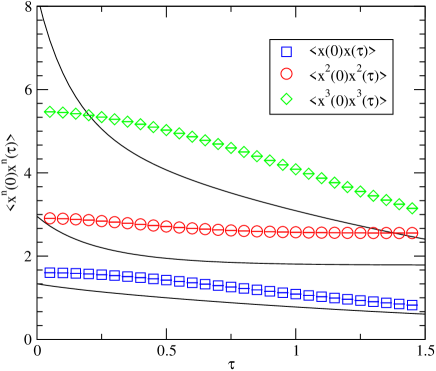
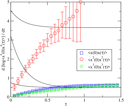
Figure 10: Same as Fig. 4 but the correlation functions are evaluated from a random instanton configuration.

Given the success of the semi-classical approximation in predicting the splitting between the ground state and the first excited state it seems natural to study the correlation functions in the semi-classical approximation in more detail. We begin by considering the contribution from the classical path only. In this case the partition function is given by

$$Z=\sum_{n_{I},n_{A}}\frac{\delta_{n_{I},n_{A}}}{n_{I}!n_{A}!}\left(\prod_{i}\int d\tau_{i}\right)\exp(-S).$$ (30)

Here, $n_{I},n_{A}$ are the number of instanton and anti-instantons, $\tau_{i}$ are the (anti) instanton positions, and $S_{0}$ is the classical action. In the next section we will discuss the problem of choosing the correct path for a multi-instanton configuration in more detail. The simplest choice is the sum ansatz given in equ. (27). The coordinate correlation function is given by

$$\Pi_{cl}(\tau)=\langle x_{cl}(0)x_{cl}(\tau)\rangle,$$ (31)

where $\langle.\rangle$ denotes an ensemble average over the collective coordinates $\tau_{i}$. The distribution of collective coordinates is controlled by the partition function equ. (30). The simplest approximation is to ignore the interaction between instantons. In this case the action is $S=(n_{I}+n_{A})S_{0}$ and the distribution of collective coordinates is random. This is known as the instanton gas model or the random instanton approximation.

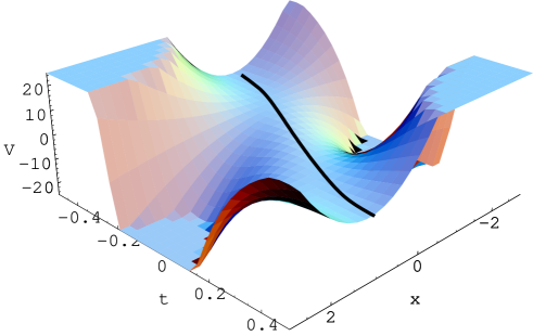
Figure 11: Gaussian effective potential for small fluctuations around a single instanton path centered at $\tau=0$.

Correlation functions in a random instanton gas are shown in Fig. 10. We note that the result is very similar to the cooled correlation functions shown in Fig. 6. This is in agreement with our earlier observation that the cooled configurations are very close to a simple superposition of instantons. Like the the cooling calculation the random instanton gas reproduces the splitting between the ground state and the first excited state, but it does not give a good description of other aspects of the correlation functions.

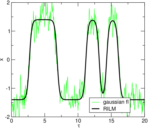
Figure 12: Typical random instanton configuration and the same configuration with Gaussian fluctuations. The noisy path was generated using 10 heating sweeps in the Gaussian potential around the classical path. This figure should be compared with Fig. 2.

It is clear that the main feature that is missing from the ensemble of classical paths is quantum fluctuations. Quantum fluctuations appear at next order in the semi-classical approximation. We already noted that quantum fluctuations determine the pre-exponential factor in the tunneling rate, see equ. (26). We can write the path as $x(\tau)=x_{cl}(\tau)+\delta x(\tau)$ where $x_{cl}(\tau)$ is the classical path and $\delta x(\tau)$ is the fluctuating part. To second order in $\delta x$ the action is given by equ. (28). For a single instanton it is possible to determine the propagator $\langle\delta x(0)\delta x(\tau)\rangle$ analytically, see equ. (39) in Schafer:1996wv . For an ensemble of instantons we can approximate the propagator as a sum of contributions due to individual instantons. This is the procedure that is used in the QCD calculations described in Shuryak:1992jz ; Shuryak:1992ke ; Schafer:1995pz ; Schafer:1995uz .

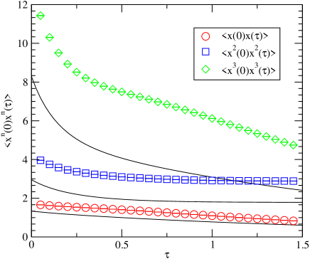
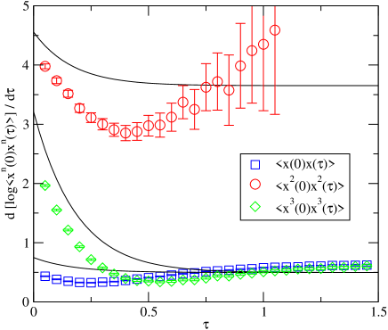
Figure 13: Same as Fig. 4 but the correlation functions are evaluated in a random instanton ensemble with Gaussian fluctuations.

Alternatively, we can determine the correlation function numerically, using the “heating” method. As the name suggests, this is essentially the inverse of the cooling method. We begin from a classical path and determine the Gaussian effective potential for small fluctuations around the path. For a single instanton, the action is given by

$$S=\int d\tau\,\left(\frac{1}{4}\delta\dot{x}^{2}(\tau)+4\eta^{2}\left[1-\frac{3}{2\cosh^{2}(2\eta(\tau-\tau_{I}))}\right]\delta x^{2}(\tau)\right),$$ (32)

see Fig. 11. This action has one zero mode $\delta x(\tau)=-S_{0}^{-1/2}dx_{cl}(\tau-\tau_{I})/(d\tau_{I})$ which corresponds to translations of the instanton solution. We can eliminate the corresponding non-Gaussian fluctuations by imposing a constraint on the location of the instanton. Using the simple identity

$$1=\int d\tau_{I}\,\delta(x(\tau_{I}))\,\left|\dot{x}(\tau_{I})\right|$$ (33)

we see that the corresponding Jacobian is the velocity $\dot{x}(\tau_{I})$. We can now perform Monte Carlo calculations using the Gaussian action for a multi-instanton configuration. The method is illustrated in Fig. 12. The black line shows the classical path and the green path is the same path with Gaussian fluctuations included. Clearly, this path looks very similar to the full quantum path shown in Fig. 2. There are still some differences, however. We notice, in particular, that the fluctuations around the minima of the potential are not completely symmetric. This is related to non-Gaussian effects. We also observe that the heated random instanton path lacks large excursions from the minima of the potential that do not lead to a tunneling event. These effects are due to a combination of instanton interactions and large non-Gaussian effects.

Correlation functions in the random instanton configurations with Gaussian fluctuations included are shown in Fig. 13. We observe that the correlation functions are in much better agreement with the exact results than the correlators obtained from the classical path only. We also see that the correlators not only describe the splitting between the ground state and the first excited state but also provide a reasonable description of the second excited state.

VIII Instanton interactions

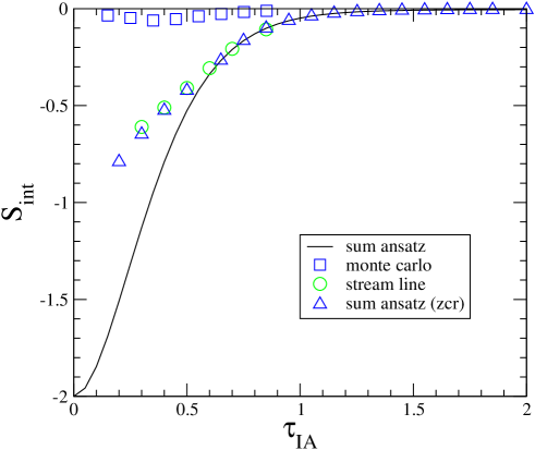
Figure 14: Instanton-anti-instanton interaction in units of $S_{0}$ as a function of the instanton-anti-instanton separation. The solid line shows the result in the sum ansatz. The triangles show the same data plotted as a function of the zero crossing distance. The streamline interaction is shown as the circles and the squares show the effective interaction extracted from the cooled intanton-anti-instanton distribution shown in Fig. 16.

Another feature that is missing from the random instanton ensemble is the correlation between tunneling events due to the interaction between instantons. In QCD instanton interactions, in particular those mediated by fermions, are very important and lead to qualitative changes in the instanton ensemble. In the quantum mechanical model studied here the interaction between instantons is short range and only leads to relatively small effects. These effects can nevertheless be clearly identified in very accurate calculations. We refer to Schafer:1996wv for a discussion of the contribution of instanton-anti-instanton pairs to the ground state energy.

The simplest method for studying the instanton-anti-instanton interaction is to construct a trial function and compute its action. For the sum ansatz given in equ. (27) the result is shown as the solid line in Fig. 14. Asymptotically, the action is given by $S_{IA}(\tau_{IA})=2S_{0}(1-6\exp(-\eta\tau_{IA})+\ldots)$ where $\tau_{IA}=|\tau_{I}-\tau_{A}|$ is the instanton-anti-instanton separation. In the opposite limit, $\tau_{IA}\to 0$, the instanton and anti-instanton annihilate and the action tends to zero. It is clear, however, that in this limit the sum ansatz is at best an approximate solution to the classical equation of motion, and it is not obvious how the path should be chosen.

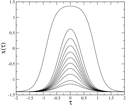
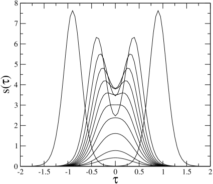
Figure 15: Solution of the streamline equation for an instanton-anti-instanton pair. Figure a shows the streamline path and the Fig. b shows the action density. The paths correspond to $S/S_{0}=2.0,1.8,\ldots,0.2,0.1$.

The best way to deal with this problem is the “streamline” or “valley” method Balitsky:1986qn ; Verbaarschot:1991sq . The method is based on the observation that in the space of all instanton-anti-instanton paths there is one almost flat direction along which the action slowly varies between $2S_{0}$ and 0. All other directions correspond to perturbative fluctuations. We can force the instanton-anti-instanton path to descend along the almost flat direction by adding a constraint

$$S_{\xi}=\xi(\lambda)\int d\tau\,\left(x(\tau)-x_{\lambda}(\tau)\right)\frac{dx_{\lambda}(\tau)}{d\lambda}$$ (34)

to the classical action. Here, $\lambda$ labels the different instanton-anti-instanton paths along the streamline and $\xi(\lambda)$ is a Lagrange multiplier. We find the streamline configuration by starting from a well separated IA pair and letting the system evolve using the method of steepest descent. This means that we have to solve

$$\xi(\lambda)\frac{dx_{\lambda}(\tau)}{d\lambda}=\left.\frac{\delta S}{\delta x(\tau)}\right|_{x=x_{\lambda}},$$ (35)

with the boundary condition that $x_{\lambda=0}(\tau)\simeq x_{sum}(\tau)$ corresponds to a well separated instanton-anti-instanton pair. Note that $\xi(\lambda)$ is an arbitrary function that reflects the reparametrization invariance of the streamline solution. A sequence of paths obtained by solving equ. (35) numerically is shown in Fig. 15. We also show the action density $s=\dot{x}^{2}/4+V(x)$. We can see clearly how the two localized solutions merge and eventually disappear as the configuration progresses down the valley.

There is no unique way to parametrize the streamline path and extract the instanton-anti-instanton action as a function of the separation between the tunneling events. The simplest possibility is to used the distance between the zero crossings $\tau_{z}$. This definition has the advantage of being very easy to use, but it prevents us from exploring the part of the streamline trajectory where the instanton and anti-instanton are so close that the path never crosses zero. In Fig. 14 we compare results for $S_{IA}(\tau_{z})$ obtained from the sum ansatz and the streamline solution. We observe that for instanton separations $\tau_{z}>0.3$ the results are very similar. We also note, however, that for $\tau_{z}<0.6$ the zero crossing distance is quite different from the parameter $\tau_{I}-\tau_{A}$ that appears in the sum ansatz.

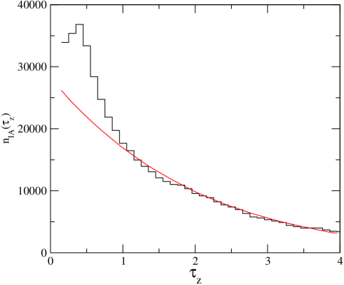
Figure 16: Distribution of instanton-anti-instanton separations after 10 cooling sweeps. The separation was extracted from the distance of the zero-crossings in the cooled configuration.

One can show that the ambiguities that arise in trying to define the instanton-anti-instanton interaction at short distance correspond to similar ambiguities that arise in the perturbative expansion because and are related to the factorial growth of higher order terms in the expansion. Only the sum of the perturbative and the instanton contribution is well defined and leads to unique predictions for the groundstate energy. In these lectures we shall not discuss this problem any further. Instead, we will study the question whether the full quantum configurations contain evidence of the correlations between instantons that the classical instanton-anti-instanton interaction implies.

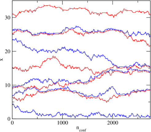
Figure 17: Typical instanton configuration in an interacting instanton calculation. The figure shows the location $x$ of the first 10 instantons (blue) and anti-instantons (red) over a period of 3000 configurations.

In Fig. 16 we show a histogram of the instanton-anti-instanton separation determined in Monte Carlo simulations of the quantum mechanical partition function. The data were obtained by measuring the zero crossing distance after 10 cooling sweeps. For comparison we also show the $IA$ distribution in the random instanton gas. We observe that there is an enhancement of close $IA$ pairs which corresponds to an attractive instanton-anti-instanton interaction. The exact magnitude of this enhancement depends sensitively on the number of cooling sweeps. As emphasized in the previous paragraph, this is not necessarily a shortcoming of the cooling method. We can try to translate the enhancement in the $IA$ distribution into an effective interaction using the classical relation $n(\tau_{IA})\sim n_{0}(\tau_{IA})\exp(-S_{IA}(\tau_{IA}))$. Here, $n(\tau_{IA})$ is the $IA$ distribution, $n_{0}(\tau_{IA})$ is the distribution in the random theory and $S_{IA}(\tau_{IA})$ is the instanton-anti-instanton interaction. The result is also shown in Fig. 14. We observe that the interaction extracted from the $IA$ distribution is significantly weaker than the classical result. This may imply that the full quantum interaction is weaker than the classical result, or that too many close pairs are lost during cooling. This question can be studied in more detail using the methods discussed in Sect. VI.

Finally, we address the question how to include correlations between tunneling events in the instanton calculation. For this purpose we include the instanton-anti-instanton interaction in the instanton liquid partition function equ. (30). In this context we again have to address the problem of close instanton-anti-instanton pairs. The simplest approach is to add a short range repulsive core which excludes configurations that are not semi-classical. The hard core interaction can be adjusted in order to reproduce the $IA$ distribution found in the cooling calculation. In practice we have chosen $S_{core}(\tau_{IA})=A_{c}\exp(-\tau_{IA}/\tau_{c})$ with $A_{c}=3$ and $\tau_{c}=0.3$. In Fig. 17 we show a typical set of instanton and anti-instanton trajectories from an interacting instanton calculation. Correlations between instantons are clearly visible. In particular, we observe that a number of close instanton-anti-instanton pairs are formed. We have also studied correlation functions in the interacting instanton ensemble. We find that differences as compared to the random ensemble are rather subtle and a detailed study of non-Gaussian effects is necessary in order to establish the importance of instanton interactions.

IX Summary

In these lectures we presented Monte Carlo methods for studying the euclidean path integral in Quantum Mechanics. We also supply a set of computer codes written in fortran that were used to generate the data shown in the figures. We encourage the reader to play around with these programs in order to get a deeper appreciation of the path integral and of Monte Carlo methods.

We should note that Monte Carlo calculations of the euclidean path integral are an extremely poor way to compute the spectrum or the correlation functions of the anharmonic oscillator. The code based on diagonalizing the Hamiltonian is both much faster and much more accurate than the Monte Carlo codes. The purpose of the Monte Carlo codes is entirely pedagogical. However, if we proceed from quantum mechanics to systems involving many more degrees of freedom, such as four-dimensional field theories, Hamiltonian methods become more and more impractical and Monte Carlo calculations based on the euclidean path integral provide the most efficient method for computing the spectrum and the correlation functions known to date.

We also discussed Monte Carlo methods for studying the contribution of instantons to the euclidean path integral. In the case of the double well potential there is a parameter, $\eta$, which controls the instanton action $S_{0}=4\eta^{3}/3$. If $S_{0}\gg 1$ then instantons are easily identified but the tunneling rate is small. If $S_{0}\sim 1$ then instantons are very abundant but it is hard to determine the instanton density precisely. We focused on the case $S_{0}\sim 3$ which is at the boundary of the semi-classical regime. Even though the expansion parameter $1/S_{0}$ is not very small the instanton density is still well determined and agrees with the level splitting. We also noticed, however, that non-Gaussian effects are important in this regime.

Ultimately, we are interested in the question to what extent these results can be generalized to QCD. In QCD there is no free parameter that controls the applicability of the semi-classical expansion. Unlike the case of the double well potential, instantons in QCD can have any size. Asymptotic freedom implies that the action of small instantons is big, but the action of instantons with size $\rho\sim\Lambda_{QCD}^{-1}$ is of order one. Nevertheless, lattice calculations support the idea that the tunneling density is sizable, $(N/V)\simeq\Lambda_{QCD}^{4}\simeq 1\,{\rm fm}^{-4}$, and that instantons do not strongly overlap Chu:1994vi . The typical instanton size is found to be $\rho\sim(0.3-0.4)$ fm which implies a typical instanton action $S_{0}\simeq(5-10)$. The reason that the density is big even though the action is significantly larger than one is related to the fact that QCD instantons have many more collective coordinates, 12 (4 coordinates, 1 size, 7 color angles) compared to just one in the case of the double well potential. As a consequence the pre-exponential factor in the tunneling rate is numerically large.

There are some important differences between QCD and the double well potential. In a typical lattice QCD configuration quantum fluctuations of the gauge field are much bigger than the classical gauge fields associated with instantons. This implies that one cannot “see” instantons in the gauge configurations in the same way that one can immediately identify tunneling events in the quantum mechanical paths. Compare, for example, Fig. 2 with Fig. 1 in Chu:1994vi . Only after some amount of cooling do instantons emerge from the quantum noise. On the other hand, fermions provide an important diagnostic tool in QCD that is not available in the simple bosonic model analyzed in these lectures. Instantons lead to localized chiral zero modes of the Dirac operators that can easily be identified even in noisy quantum configurations.

Appendix A Computer Codes

All programs are written in standard fortran 77, have extensive comments and do not require any libraries. Some of the programs contain subroutine for generating random numbers or for diagonalizing matrices that were taken from Numerical Recipes (Numerical Recipes in Fortran, W. H. Press, S. A. Teukolsky, W. T. Vetterling and B. D. Flannery, Cambridge University Press).

1. qmdiag.for

This programs computes the spectrum and the eigenfunctions of the anharmonic oscillator. The results are used in order to compute euclidean correlation functions.

Input: fort.05

$f$	minimum of anharmonic oscillator potential $V(x)=(x^{2}-f^{2})^{2}$
$N$	dimension of basis used for diagonalizing $H$ (choose $N\geq 40$)
$\omega_{0}$	unperturbed oscillator frequency (choose $\omega_{0}\sim 4f$)

Output: qmdiag.dat

$E_{n}$	eigenvalue of Hamiltonian
$c_{n}$	dipole matrix element $c_{n}^{2}=|\langle 0|x|n\rangle|^{2}$
$d_{n}$	quadrupole matrix element $d_{n}^{2}=|\langle 0|x^{2}|n\rangle|^{2}$
$e_{n}$	quadrupole matrix element $d_{n}^{2}=|\langle 0|x^{3}|n\rangle|^{2}$
$\psi(x)$	ground state wave function
$\langle x(0)x(\tau)\rangle$	euclidean correlation function, also for $x^{2}$ and $x^{3}$
$d\log\Pi/(d\tau)$	log derivative of $\Pi(\tau)=\langle x(0)x(\tau)\rangle$
$Z(\beta)$	partition function

2. qm.for

This programs computes correlation functions of the anharmonic oscillator using Monte Carlo simulations on a euclidean lattice.

Input: fort.05

$f$	minimum of anharmonic oscillator potential $V(x)=(x^{2}-f^{2})^{2}$
$n$	number of lattice points in the euclidean time direction ($n\sim 800$)
$a$	lattice spacing ($a\sim 0.05$)
$ih$	$ih=0$ cold start $x_{i}=-f$, $ih=1$ hot start $x_{i}=ran()$
$n_{eq}$	number of equilibration sweeps before first measurement $(n_{eq}\sim 100)$
$n_{mc}$	number of Monte Carlo sweeps ($n_{mc}\sim 10^{5}$)
$\delta x$	width of Gaussian distribution used for Monte Carlo update $x_{i}^{(n)}\to x_{i}^{(n+1)}$ ($\delta x\sim 0.5$)
$n_{p}$	number of points on which correlation functions are measured $\langle x_{i}x_{i+1}\rangle,\ldots,$ $\langle x_{i}x_{i+n_{p}}\rangle$ $(n_{p}\sim 20)$
$n_{mea}$	number of measurements of the correlation function in a given Monte Carlo configuration ${x_{i}}$ ($n_{mea}\sim 5$)
$n_{pri}$	number of Monte Carlo configurations between output of averages to output file ($n_{pri}\sim 100$)

Output: qm.dat

$S_{tot}$	average total action per configuration
$V_{av},T_{av}$	average potential and kinetic energy
$\langle x^{n}\rangle$	expectation value $\langle x^{n}\rangle$ ($n=1,\ldots,4$)
$\Pi(\tau)$	euclidean correlation function $\Pi(\tau)=\langle O(0)O(\tau)\rangle$ for $O=x$, $x^{2}$, $x^{3}$. Results are given in the format $\tau,\Pi(\tau)$, $\Delta\Pi(\tau)$, $d\log(\Pi)/(d\tau)$, $\Delta[d\log(\Pi)/(d\tau)]$, where $\Delta\Pi(\tau)$ is the statistical error in $\Pi(\tau)$.

3. qmswitch.for

The program qmswicth.for computes the free energy $F=-T\log(Z)$ of the anharmonic oscillator using the method of adiabatic switching between the harmonic and the anharmonic oscillator. The action is $S_{\alpha}=S_{0}+\alpha(S-S_{0})$. The code switches from $\alpha=0$ to $\alpha=1$ and then back to $\alpha=0$. Hysteresis effects are used in order to estimate errors from incomplete equilibration. Most input parameters are the same as in qm.for. Additional parameters are given below.

Input: fort.05

$\omega_{0}$	oscillator constant of the reference system ($\omega_{0}\sim 4f$)
$n_{switch}$	number of steps in adiabatic switching ($n_{switch}\sim 20$)

Output: qmswitch.dat

The output file contains many details of the adiabatic switching procedure. The final result for the free energy is given as $F=F_{0}+\delta F$, where $F_{0}$ is the free energy of the harmonic oscillator and $\delta F$ is the integral over $\alpha$. We estimate the uncertainty in the final result as $F\pm\Delta F(stat)\pm\Delta F(equ)\pm\Delta F(disc)$, where $\Delta F(stat)$ is the statistical error, $\Delta F(equ)$ is due to incomplete equilibration (hysteresis), and $\Delta F(disc)$ is due to discretizing the $\alpha$ integral.

4. qmcool.for

This programs is identical to ${\tt qm.for}$ except that expectation values are measured both in the original and in cooled configurations. We only specify additional input parameters.

Input: fort.05

$n_{st}$	number of Monte Carlo configurations between successive cooled configurations. The number of cooled configurations is $n_{conf}/n_{st}$ ($n_{st}\sim 20$).
$n_{cool}$	number of cooling sweeps ($n_{cool}\sim 50$)

Output: qmcool.dat

$\Pi(\tau)$	correlation functions are given in the same format as in ${\tt qm.dat}$
$N_{I+A}$	total number of instantons extracted from number of zero crossings
	as a function of the number of cooling sweeps
$S_{tot}$	total action vs number of cooling sweeps
$S/N$	action per instanton. $S_{0}$ is the continuum result for one instanton

5. qmidens.for

The program qmidens.for calculates non-Gaussian corrections to the instanton density using adiabatic switching between the Gaussian action and the full action. The calculation is performed in both the zero and one-instanton-sector. The details of the adiabatic switching procedure are very similar to the method used in qmswitch.for. Note that the total length of the euclidean time domain, $\beta=na$, cannot be chosen too large in order to suppress transitions between the one-instanton sector and the three, five, etc. instanton sector. Most input parameters are defined as in qm.for.

Input: fort.05

$n_{switch}$

number of steps in adiabatic switching ($n_{switch}\sim 20$)

Output: qmidens.dat

The output file contains many details of the adiabatic switching procedure. The final result for the instanton density is compared to the Gaussian (one-loop) approximation. Note that the method breaks down if $f$ is too small or $\beta$ is too large.

6. rilm.for

This program computes correlation functions of the anharmonic oscillator using a random ensemble of instantons. The multi-instanton configuration is constructed using the sum ansatz. Note that, in contrast to RILM calculations in QCD, the fields and correlation functions are computed on a lattice.

Input: fort.05

$f$	minimum of anharmonic oscillator potential $V(x)=(x^{2}-f^{2})^{2}$
$n$	number of lattice points in the euclidean time direction ($n\sim 800$)
$a$	lattice spacing ($a\sim 005$)
$N_{I+A}$	number of instantons (has to be even). The program displays the one and two-loop result for the parameters $(f,\beta=na)$.
$n_{mc}$	number of configurations ($n_{mc}\sim 10^{3}$)
$n_{p}$	number of points on which correlation functions are measured $\langle x_{i}x_{i+1}\rangle,\ldots,$ $\langle x_{i}x_{i+n_{p}}\rangle$ $(n_{p}\sim 20)$
$n_{mea}$	number of measurements of the correlation function in a given Monte Carlo configuration ${x_{i}}$ ($n_{mea}\sim 5$)
$n_{pri}$	number of Monte Carlo configurations between output of averages to output file ($n_{pri}\sim 100$)

Output: rilm.dat

$S_{tot}$	average total action per configuration.
$V_{av},T_{av}$	average potential and kinetic energy.
$\langle x^{n}\rangle$	expectation value $\langle x^{n}\rangle$ ($n=1,\ldots,4$)
$\Pi(\tau)$	euclidean correlation function $\Pi(\tau)=\langle O(0)O(\tau)\rangle$ for $O=x$, $x^{2}$, $x^{3}$. Results are given in the format $\tau$, $\Pi(\tau)$, $\Delta\Pi(\tau)$, $d\log(\Pi)/(d\tau)$, $\Delta[d\log(\Pi)/(d\tau)]$.

7. rilm_gauss.for

This program generates the same random instanton ensemble as rilm.for but it also includes Gaussian fluctuations around the classical path. This is done by performing a few heating sweeps in the Gaussian effective potential. Most input parameters are defined as in rilm.for. Additional input parameters are given below.

Input: fort.05

$n_{heat}$	number of heating steps ($n_{heat}\sim 10$)
$\delta x$	coordinate update ($\delta x\sim 0.5$)

8. iilm.for

This program computes correlation functions of the anharmonic oscillator using an interacting ensemble of instantons. The multi-instanton configuration is constructed using the sum ansatz. The configuration is discretized on a lattice and the total action is computed using the discretized lattice action. Very close instanton-anti-instanton pairs are excluded by adding an nearest neighbor interaction with a repulsive core. Most input parameters are the same as in ${\tt rilm.for}$. Additional input parameters are

Input: fort.05

$\tau_{core}$	range of hard core interaction ($\tau_{core}\sim 0.3$)
$A_{core}$	strength of hard core interaction ($A_{core}\sim 3.0$)
$dz$	average position update ($dz\sim 1$)

References

- (1) A. M. Polyakov, Nucl. Phys. B 120, 429 (1977).
- (2) A. I. Vainshtein, V. I. Zakharov, V. A. Novikov and M. A. Shifman, ABC Of Instantons, Sov. Phys. Usp. 24, 195 (1982); also in ITEP Lectures on Particle Physics and Field theory, World Scientific, Singapore (1999).
- (3) S. Coleman, The Uses Of Instantons, Lecture delivered at 1977 Int. School of Subnuclear Physics, Erice, Italy (1977); also in Aspects of Symmetry, Cambridge University Press (1985).
- (4) E. V. Shuryak, The QCD Vacuum, Hadrons And The Superdense Matter, World Scientific, Singapore (1988).
- (5) H. Kleinert, Path integrals in quantum mechanics, statistics, and polymer physics, World Scientific, Singapore (1995).
- (6) J. Zinn-Justin, Quantum field theory and critical phenomena, Oxford University Press (1993).
- (7) T. Schäfer and E. V. Shuryak, Rev. Mod. Phys. 70, 323 (1998), [hep-ph/9610451].
- (8) H. Forkel, preprint, hep-ph/0009136.
- (9) R. P. Feynman, A. R. Hibbs, Quantum Mechanics and Path Integrals, McGraw-Hill, New York (l965).
- (10) M. Creutz and B. Freedman, Annals Phys. 132, 427 (1981).
- (11) E. V. Shuryak and O. V. Zhirov, Nucl. Phys. B 242, 393 (1984).
- (12) E. V. Shuryak, Nucl. Phys. B 302, 621 (1988).
- (13) M. Asakawa, T. Hatsuda and Y. Nakahara, Prog. Part. Nucl. Phys. 46, 459 (2001) [hep-lat/0011040].
- (14) M. Jarrell, and J. E. Gubernatis, Phys. Rep. 269, 133 (1996).
- (15) C. F. Wohler and E. V. Shuryak, Phys. Lett. B 333, 467 (1994) [hep-ph/9402287].
- (16) J. Hoek, Phys. Lett. B 166, 199 (1986).
- (17) J. Hoek, M. Teper and J. Waterhouse, Phys. Lett. B 180, 112 (1986).
- (18) E. V. Shuryak and J. J. M. Verbaarschot, Nucl. Phys. B 410, 37 (1993) [hep-ph/9302238].
- (19) E. V. Shuryak and J. J. M. Verbaarschot, Nucl. Phys. B 410, 55 (1993) [hep-ph/9302239].
- (20) T. Schäfer and E. V. Shuryak, Phys. Rev. D 53, 6522 (1996) [hep-ph/9509337].
- (21) T. Schäfer and E. V. Shuryak, Phys. Rev. D 54, 1099 (1996) [hep-ph/9512384].
- (22) I. I. Balitsky and A. V. Yung, Phys. Lett. B 168, 113 (1986).
- (23) J. J. M. Verbaarschot, Nucl. Phys. B 362, 33 (1991) [Erratum-ibid. B 386, 236 (1992)].
- (24) M. C. Chu, J. M. Grandy, S. Huang and J. W. Negele, Phys. Rev. D 49, 6039 (1994) [hep-lat/9312071].