Lattice QCD with two dynamical flavors of domain wall fermions

Abstract

We present results from the first large-scale study of two flavor QCD using domain wall fermions (DWF), a chirally symmetric fermion formulation which has proven to be very effective in the quenched approximation. We work on lattices of size $16^{3}\times 32$, with a lattice cut-off of $a^{-1}\approx 1.7$ GeV, and dynamical (or sea) quark masses in the range $m_{strange}/2\mathrel{\hbox to0.0pt{\raise 2.20013pt\hbox{$<$}\hss}{\lower 2.20013pt\hbox{$\sim$}}}m_{sea}\mathrel{\hbox to0.0pt{\raise 2.20013pt\hbox{$<$}\hss}{\lower 2.20013pt\hbox{$\sim$}}}m_{strange}$. After discussing the algorithmic and implementation issues involved in simulating dynamical DWF, we report on the low-lying hadron spectrum, decay constants, static quark potential, and the important kaon weak matrix element describing indirect CP violation in the Standard Model, $B_{K}$. In the latter case we include the effect of non-degenerate quark masses ($m_{s}\neq m_{u}=m_{d}$), finding $B_{K}^{\overline{MS}}(2\,{\rm GeV})=0.495\,(18)$.

I Introduction

An improved theoretical understanding of the non-perturbative aspects of QCD is increasingly important due to the continuing advance of experiments involving hadrons. Such understanding is an important ingredient in obtaining precise values of the parameters of the Standard Model and the search for new physics. It is also key to understanding the fundamental properties of QCD itself which are under intense investigation at BNL, Jefferson Lab, FNAL, CERN, and other places.

The fundamental theoretical tool to investigate QCD non-perturbatively is lattice QCD, the regularized field theory of QCD on a discrete Euclidean space-time lattice. Treatment of the fermion field in such a regularization has been a long-standing difficulty because flavor and chiral symmetry are badly broken in practical numerical simulations using conventional lattice fermions. A revolutionary theoretical framework to realize flavor and chiral symmetry on the lattice was constructed by KaplanKaplan (1992) and subsequently reformulated and extended in two distinct ways by Narayanan and NeubergerNarayanan and Neuberger (1993) and ShamirShamir (1993) who suggested that the new fermions be used to study vector gauge theories, and especially QCD. These new fermions, known as domain wall fermions, turned out to be in a class of lattice fermions that satisfy the Ginsparg-Wilson relationGinsparg and Wilson (1982). Later, Neuberger developed still another closely related lattice fermion called overlap fermionsNeuberger (1998).

Today, both domain wall and overlap fermions are commonly used in quenched lattice QCD simulations, those where the fermion determinant is set to one in all path integrals used to calculate expectation values. In this paper, we report on the first large scale two flavor dynamical simulations with domain wall fermions, those where the fermion determinant is included in all path integrals used to calculate expectation values. From a perturbative point of view, this is equivalent to keeping all closed fermion loop contributions (at lowest order, the hadronic vacuum polarization) to all orders in all Feynman diagrams.

To realize chiral symmetry, domain wall fermions utilize an extra fifth dimension, demanding increased computational resources that are essentially linear in this extra dimension. Nevertheless quenched QCD calculations with domain wall fermions were carried out, showing good chiral symmetry can be achieved with a practical number of lattice sites in the extra dimension ($L_{s}\sim 10$) Blum and Soni (1997a, b); Aoki et al. (2000). Subsequently, within the quenched approximation domain wall fermions were used in many calculations, showing dramatic improvement in scaling toward the continuum limit over conventional formulations Ali Khan et al. (2001a); Blum et al. (2004); Ali Khan et al. (2001b); Aoki et al. (2004a); Sasaki et al. (2002), were used in pioneering calculations of weak interaction hadronic matrix elementsAli Khan et al. (2001b); Noaki et al. (2003); Blum et al. (2003), and proved efficacious in non-perturbative operator renormalization Blum et al. (2002, 2003); Aoki et al. (2004b).

As mentioned already, large scale computations using domain wall fermions have so far been restricted to the quenched approximation. The problem with such calculations is that there is no way to systematically reduce the errors due to quenching without simply performing the unquenched calculation. Past experience indicates that the size of the error ranges between 5-10% for many observables, but can be much greater, depending on the observable (the critical temperature of the hadron to quark-gluon plasma phase transition is a well known example where the quenching error is more than 40%). In Aoki et al. (2004a) the ratio of pseudoscalar decay constants in the quenched approximation was found to be $f_{K}/f_{\pi}\approx 1.13(3)$, different from the experimental value, $\approx 1.22$. On the other hand, in this work, we find $f_{K}/f_{\pi}=1.175(11)$, as discussed in Section V. Moreover, there are important physical objects, the flavor singlet mesons and scalar mesons, for example, which are believed to be very sensitive to dynamical, or sea quark effects. Ultimately, to perform accurate lattice QCD calculations these effects must be included.

Recently, large-scale dynamical fermion simulations using Wilson fermions Ali Khan et al. (2002); Aoki et al. (2003); Kaneko et al. (2004) and improved staggered fermions Davies et al. (2004); Aubin et al. (2004a) (using two light degenerate quarks and a heavier quark for the strange quark) have been reported. Both formulations break chiral symmetry and the former also breaks flavor symmetry (a severe problem, theoretically and practically). Nevertheless, calculations using either type of fermions, done with two or more sufficiently small lattice spacings, have yielded results which agree accurately with experiment for some observables. QCD simulations using staggered fermions are much less computationally demanding, making them attractive. However, the action corresponds to four degenerate fermions in the continuum limit, so to simulate a single flavor requires the fourth root of the determinant. For this to be a legitimate procedure there must be a local action for a single flavor of staggered fermions which had the same determinant as this fourth root. While there is no proof that such a decomposition is impossible, no such action has been constructed to date. The flavor symmetry breaking intrinsic to staggered fermions also leads to larger than expected discretization errors, a problem that is significantly reduced by improving the naive discretization (see Orginos and Toussaint (1999); Orginos et al. (1999); Lepage (1999)). Even with these improvements, an extended chiral perturbation theory Aubin and Bernard (2003a, b) with many extra low energy constants corresponding to the leading lattice-spacing errors must be used to do the chiral extrapolations. Without this extra complexity, the precise agreement with experiment could not be achieved without costly reductions in the lattice spacing. While more computationally demanding than staggered fermions, the Wilson fermion formulation is still much less demanding than DWF. However, this action severely breaks chiral symmetry, leading to large discretisation errors (starting at $O(a)$ rather than $O(a^{2})$ for un-improved Wilson fermions) and a problematic renormalization structure. In addition to this, the Wilson Dirac operator for a single flavor cannot be proved to have a positive determinant for positive quark mass, which is an important prerequisite for simulating an odd number of dynamical flavors exactly using the currently available algorithms.

For these reasons, full QCD simulations with DWF are necessary as they avoid these theoretical uncertainties by providing a fermion formulation with both exact flavor symmetry, and good chiral properties. In fact , in the limit of an infinite extra dimension domain wall fermions posses exact chiral symmetry at non-zero lattice spacing, that is, away from the continuum limit. When the extent of the extra dimension ($L_{s}$) is finite, explicit chiral symmetry breaking is induced and is quantified in the form of a small additive quark mass $m_{res}$. The domain wall fermion Dirac operator has the nice property that for positive mass and even $L_{S}$ its determinant is positive, and so taking the square-root of the two flavor determinant is a well defined operation. This, in combination with algorithms such as the polynomial Aoki et al. (2002) and rational Clark et al. (2003); Clark and Kennedy (2004) hybrid Monte Carlo algorithms, allows an odd number of dynamical flavors to be simulated exactly. In addition, if the gauge fields are sufficiently smooth that the underlying Wilson-Dirac operator is not in the parity broken Aoki phase Aoki (1984)), then the theory is expected to be local. This condition has been met in quenched studies. We refer the interested reader to Golterman and Shamir (2003) and references therein for a full explanation. Note that the same locality condition applies to overlap fermions. Thus unquenched lattice QCD with domain wall, or overlap , fermions promises to be the closest non-perturbatively regularized theory to continuum QCD. This continuum-like (symmetry) property is central to the argument that despite Ginsparg-Wilson fermions being naively more expensive, superior scaling with the lattice spacing $a$ and greatly simplified renormalization structure may eventually overcome the increased computational burden since dynamical lattice simulations are known to scale as $a^{-(7-8)}$ as the continuum, chiral, and infinite lattice volume limits are approached.

Several years ago some of us performed a study of the finite temperature QCD phase transition using dynamical domain wall fermionsChen et al. (2001). Large explicit chiral symmetry breaking was evident in, for example, the quark mass dependence of the pion mass, which is now believed to be caused the gauge field being sufficiently rough that there was a condensation of zero-modes of the four-dimensional Wilson Dirac operator appearing in the domain wall fermion operator (the Aoki phase); the lattice scale in these simulations was below 1 GeV. Here we have moved to a finer lattice spacing, $a^{-1}\sim 1.7$ GeV, and use an improved gauge action which significantly reduced the explicit chiral symmetry breaking in quenched calculations by an order(s) of magnitudeAoki et al. (2004a). As discussed in Section V, $m_{res}$ is a few MeV in this calculation, so we are confident that our simulation is not inside the Aoki phase and that, in fact, explicit chiral symmetry breaking is small and under precise control for a relatively modest $L_{s}=12$. The mass of the two dynamical domain wall quarks, $m_{q}=m_{f}+m_{res}$, is roughly in the range one half to one times the strange quark mass, meaning the residual quark mass due to the finite size of the fifth dimension is a small fraction of the input quark mass.

This paper is organized as follows. The lattice action and its numerical implementation with various improvements are described in Section II. The ensemble of gauge field configurations is summarized in Section III. Thermalization and auto-correlations in simulation time are discussed in Section IV. Physical results are presented in Section V with an emphasis on an analysis to next-to-leading order in chiral perturbation theory. In section VI we discuss aspects of chiral symmetry related to domain wall fermion simulations and compare and contrast dynamical and quenched simulations. We summarize our results and conclusions in Section VII.

II Implementation of dynamical DWF

In this section we will discuss the algorithmic and implementation details involved in generating dynamical ensembles with the domain wall fermion action. As a first step we must precisely define the domain wall fermion action that we have used. For the domain wall fermion Dirac operator, $D_{\rm DWF}$, we use the same definition and conventions as Blum et al. (2004). However, were we simply to use the action $S=S_{F}+S_{G}$ with

$$S_{F}=\sum_{x}\bar{\Psi}D_{DWF}\Psi$$ (1)

and $S_{G}$ representing the gauge action (in our case the DBW2 action), then we would face a problem: the fifth direction in the domain wall fermions framework naturally gives rise to unphysical heavy propagating modes in this direction, while we are only interested in the physics of the light mode which is bound to the domain walls. The number of such modes will diverge in the $L_{s}\rightarrow\infty$ limit and so dominate the path integral. To cancel off this divergence we add a set of Pauli-Villars fields to the action such that $S=S_{F}+S_{G}+S_{PV}$ with

$$S_{PV}=\sum_{x}\Phi^{\dagger}D_{DWF}(m_{f}=1)\Phi\,.$$ (2)

Note that, while the original formulation of the domain wall fermion action included Pauli-Villars fields Furman and Shamir (1995), here we are using a slightly different form for these fields which was introduced in Vranas (1998).

To simulate dynamical fermions on the lattice we have a choice of many algorithms Gottlieb et al. (1987); Duane et al. (1987); Luscher (1994); Aoki et al. (2002); Clark et al. (2003); Clark and Kennedy (2004). As in this work we are simulating an even number of dynamical flavors, it is convenient to use the well-known, exact, hybrid Monte Carlo (HMC) $\Phi$ algorithm Gottlieb et al. (1987); Duane et al. (1987). The precise details of the HMC algorithm can be found in the cited papers, but for convenience we will sketch an overview here:

• The fermionic part of the action is rewritten in terms of a set of bosonic fields using the relation:

  $$\int[d\overline{\psi}][d{\psi}]e^{\overline{\psi}M\psi} = {\rm det}\left(M\right)$$

  $$= \int[d\phi][d\phi^{\dagger}]e^{-\phi^{\dagger}\frac{1}{M}\phi}\,.$$

  For this bosonic integral to converge the matrix, $M$, must have eigenvalues whose real parts are positive. Due to this condition this algorithm may not be applied to QCD-like theories with an odd number of flavors. However, it may be applied to theories where quark flavors appear in degenerate mass pairs. In this situation we may use the fact that

  $$\gamma_{5}RD_{DWF}R\gamma_{5}=D_{DWF}^{\dagger},$$ (4)

  where $R$ is the reflection operator in the fifth dimension, to rewrite ${\rm det}(D_{DWF})^{2}$ as ${\rm det}(D_{DWF}^{\dagger}D_{DWF})$. The matrix that will appear in the bosonic integral is therefore

  $$\frac{1}{D^{\dagger}_{DWF}D_{DWF}}$$ (5)

  which is the square of a Hermitian matrix and so is positive semi-definite.

• An auxiliary field, $P_{\mu}$, is also added to the action. This field plays the role of a conjugate momenta to the gauge field in a molecular dynamics evolution.

• The evolution of the gauge field is split up into trajectories. At the beginning of each trajectory the pseudo-fermion field, denoted $\phi$ in Equation • ‣ II, and the conjugate momenta are chosen from a heatbath. The gauge field and conjugate momenta are then evolved some distance in “molecular dynamics time” using a discretization of Hamilton’s equations, which must be reversible. Several discretization techniques exist in the literature Duane et al. (1987); Takaishi (2002); Sexton and Weingarten (1992); in this work we are mainly using that introduced in Duane et al. (1987), although we also present the results of an exploratory study of the multiple timescale technique of Sexton and Weingarten (1992).

• If the evolution of the gauge field exactly followed Hamilton’s equations then this algorithm would be complete. However, to correct for discretization errors, a Metropolis accept/reject step is performed at the end of every trajectory.

Each step in the molecular dynamics evolution requires an inversion of the domain wall Dirac operator. While we use an even-odd preconditioned form for the operator to speed this up, it is, of course, still the most expensive part of the gauge field generation. In the following subsections we give details of our attempts to minimize both the number of inversions needed, and the cost of each of these inversions.

II.1 New Force Term

The initial studies of dynamical domain wall fermions Chen et al. (2001) used separate sets of bosonic fields to simulate the fermionic and Pauli-Villars parts of the action. This is potentially wasteful, especially for a large fifth dimension, as the entire reason for including the Pauli-Villars term was to cancel much of the contribution from the domain wall fermion Dirac operator. By using disparate sets of fields this cancellation is only apparent after the average over these fields; over a single trajectory the mismatch between these two pieces of the action may introduce large forces, and therefore large time-step errors, into the molecular dynamics evolution.

In an attempt to avoid this problem we have implemented a form of the Hamiltonian for the molecular dynamics evolution, first suggested in Vranas (1998), that uses a single set of bosonic fields to estimate both the fermion and Pauli-Villars terms. To do this we simply note that

$$\frac{{\rm det}\left(D^{\dagger}(m_{f})D(m_{f})\right)}{{\rm det}\left(D^{\dagger}(1)D(1)\right)} = {\rm det}\left(D(1)\frac{1}{D^{\dagger}(m_{f})D(m_{f})}D^{\dagger}(1)\right)^{-1}$$

$$= \int[d\Phi][d\Phi^{\dagger}]e^{-S_{n}(\Phi)}$$

with

$$S_{n}=\sum_{x}\Phi^{\dagger}D(m_{f}=1)\frac{1}{D^{\dagger}(m_{f})D(m_{f})}D^{\dagger}(m_{f}=1)\Phi\,.$$ (7)

This approach needs no more memory space than the previous one and requires exactly the same number of Dirac operator inversions as before, although they are performed on different sources. However, the cancellation between the fermion and Pauli-Villars contributions to the molecular dynamics force now happens exactly, step-by-step in the leapfrog evolution, rather than stochastically.

Table 1 gives the parameters for, and results of, a small volume head-to-head comparison of the old and new force terms on an $8^{3}\times 4\times 8$ ( where the parameters are spatial volume times temporal length times $L_{s}$) lattice using the Wilson gauge action with $\beta=5.2$, and $N_{f}=2$ domain wall fermions with $m_{f}=0.02$. As can be seen the new force term has both a significantly higher acceptance than the old force term when compared at the same step size, and a (small) reduction in the number of conjugate gradient iterations needed. The difference of the Hamiltonian used in the molecular dynamics evolution between the first and the last configuration in a trajectory, $\Delta H$, is also measured. We find the theoretical relation to the acceptanceGupta et al. (1990); Takaishi (2002),

$${\rm Prob}_{acc}\cong{\rm erfc}\left(\sqrt{\left\langle\Delta H\right\rangle}/2\right)\cong\exp\left(-\frac{\sqrt{\left\langle(\Delta H)^{2}\right\rangle}}{2\pi}\right)\ ,$$ (8)

holds to a good accuracy. For large space-time volume, $V$, and small size, $\Delta t$, the scaling

$$\sqrt{(\Delta H)^{2}}=C_{\Delta H}(\Delta t)^{2}\sqrt{V}~{}~{},$$ (9)

is expected, where the coefficient, $C_{\Delta H}$, is independent of volume and step size at leading order. By switching to the new force term, $C_{\Delta H}$ is reduced by more than a factor of two, leading to an increased acceptance, as seen in Table 1.

A similar or somewhat better reduction of the discretization error of the new force term is observed for the larger lattices ($16^{3}\times 32\times 12$) and smaller couplings on which we base much of this work. A detailed description of the basic parameters for these ensembles is deferred until Section III; here we give only the details relevant for the HMC evolution which are summarized in Table 2. We also present the results of a short test using the old force term for 45 trajectories, starting from the thermalized lattice of the lightest sea quark mass. Using the new force term, $C_{\Delta H}$ is reduced to to $\sim$ 40% of it’s value with the old force term, and the acceptance is increased from 56% to 77%, as shown in Table 2. An important observation is that $C_{\Delta H}$ is almost independent of the sea quark mass for the new force term in our simulation. This is in contrast to the empirical assumption Christ (2002); Ukawa (2002), $C_{\Delta H}\propto m_{\rm sea}^{-\alpha}$, $\alpha\sim 2$.

In Section II.3 we will discuss a technique that allows us to exploit this new force term even more succesfully.

II.2 Chronological Invertor

For the inversion of the Dirac operator in each molecular dynamics (MD) step (the most time consuming procedure in the calculation) we use chronological invertor technique of Brower et al. (1997). We employ the conjugate gradient algorithm to find an approximate solution, $\chi$, of the inverse of the matrix $\tilde{D}^{\dagger}D$ (here $\tilde{D}$ represents the even-odd preconditioned Dirac operator), acting on the source vector, $\Psi_{F}$, by iteratively minimizing

$$\chi^{\dagger}\tilde{D}^{\dagger}\tilde{D}\chi-\chi^{\dagger}\Psi_{F}-\Psi^{\dagger}_{F}\chi\,,$$ (10)

starting from an initial guess. In the chronological invertor technique this starting vector is forecast by minimizing Equation 10 in the subspace spanned by the set of solutions from previous leapfrog steps . The precise solution is calculated by the conjugate gradient (CG) algorithm starting from this forecast, so the number of CG iterations is reduced. In this sub-section we will continue to discuss the even-odd preconditioned form of the operator.

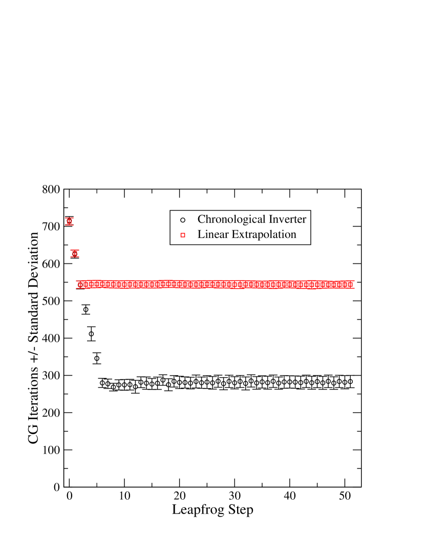
Figure 1: Conjugate gradient iteration count for the chronological inverter using the previous 7 vectors compared with a linear extrapolation of the previous two vectors for the $m_{\rm sea}=0.02$ ensemble.

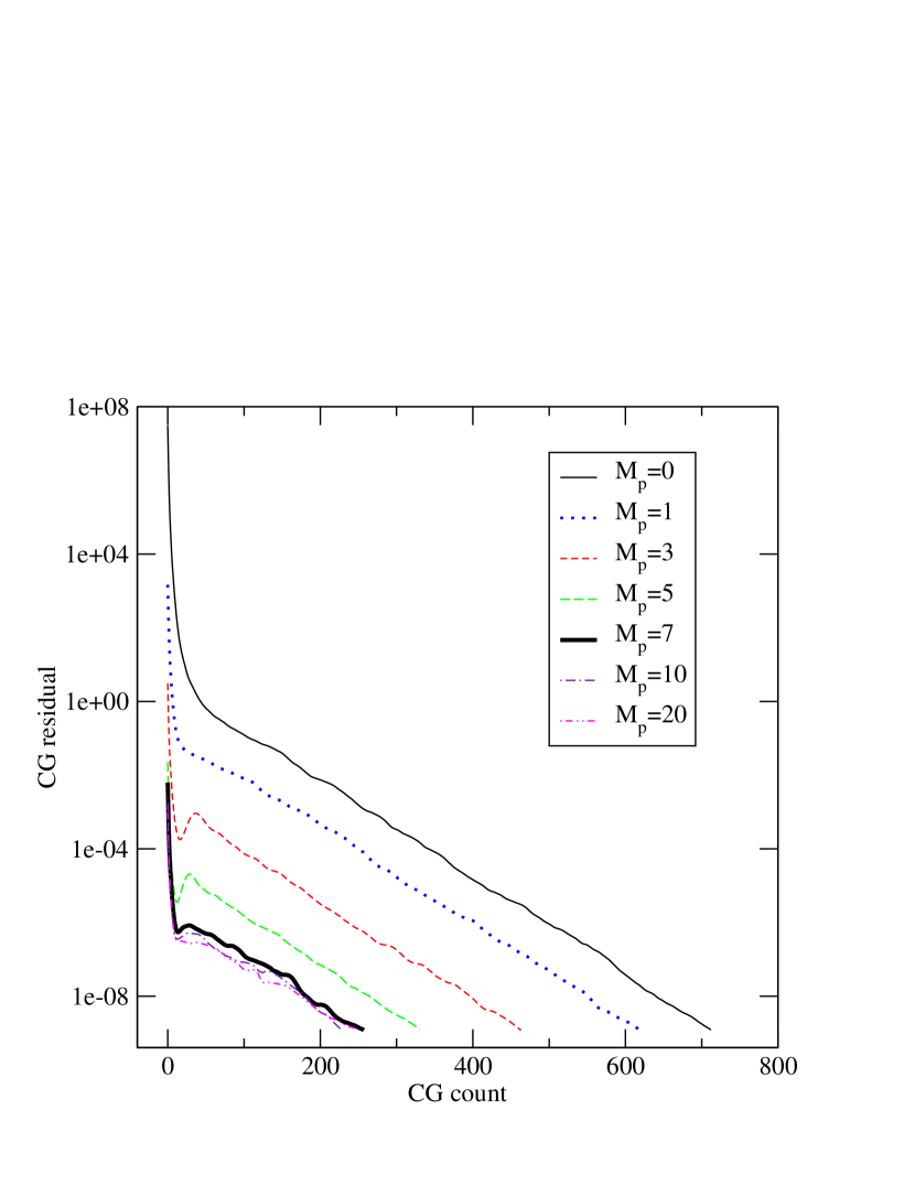
Figure 4: The residues of CG, Eq. 11, as a function of the number of CG iteration are plotted for various numbers of previous solutions, $N_{p}$, on a typical configuration of the $m_{\rm sea}=0.02$ ensemble.

The first 655 trajectories in the $m_{\rm sea}=0.02$ evolution described in Table 2 were generated using a simple linear extrapolation of the previous two solution vectors as an initial guess for the conjugate gradient algorithm Duane et al. (1987), after which we moved to the chronological invertor using the previous seven vectors (we found little advantage to using more than this number, as explained below). Figure 1 shows the average and standard deviation of the conjugate-gradient iteration count versus the leapfrog integration step for trajectories 500 to 655 and 3000 to 4000. The reduction in the number of CG iterations needed when using the chronological invertor being readily apparent. (Note: while the number of inversions is 52, the first and last of these are half-steps so the total distance moved in molecular dynamics time is $51/100$). There is, however, the overhead involved in implementing the chronological forecast. A comparison of the time taken for producing a single trajectory in our particular implementation shows roughly a factor of two speed-up whereas the CG iteration count is reduced from that without forecasting by a factor of 2.6(1), 3.2(2), 3.3(2) for the $m_{\rm sea}=0.02,$ $0.03$ and $0.04$ evolutions, respectively. Table 3 summarizes the number of CG iterations for the first 15 steps of the molecular dynamics trajectory for $m_{\rm sea}=0.02$, $m_{\rm sea}=0.03$, and $m_{\rm sea}=0.04$, together with the total number of CG iterations per trajectory. How the CG converges to the precise solution on a typical configuration of the $m_{\rm sea}=0.02$ enemble is illustrated in Figure 4 for various numbers of previous solutions, $N_{p}$, used in the forecast. The precision of the forecast is improved by increasing $N_{p}$. Since the improvement is saturated for $N_{p}\geq 7$ for all sea quark masses used, we carried out our simulation with $N_{p}=7$.

Using the chronological invertor technique, we must be careful to preserve reversibility of the MD evolution, which is a condition for the HMC algorithm to satisfy detailed balance. To be precise, a trajectory starts with a gauge configuration and its conjugate momentum, $(U^{(I)}_{\mu}(x),P^{(I)}_{\mu}(x))$, and evolves to another pair, $(U^{(F)}_{\mu}(x),P^{(F)}_{\mu}(x))$, at the end of the trajectory. Starting another evolution with the latter pair with flipped momentum, $(U^{(F)}_{\mu}(x),-P^{(F)}_{\mu}(x))$, the counterpart of the first configuration, $(U^{\prime(I)}_{\mu}(x),-P^{\prime(I)}_{\mu}(x))$, is produced. We require that $U^{\prime(I)}_{\mu}(x)$ is the same as $U^{(I)}_{\mu}(x)$ to satisfy detailed balance.

Exact reversibility is broken in two ways in the numerical simulation. Due to round-off errors, the gauge links become non-unitary and are reunitarized at the end of each trajectory. This is not a reversible process, but only causes small changes in the link elements for the parameters employed in this simulation (This statement quantified below). As mentioned previously, a more worrying source of irreversibility is the chronological invertor. Unless the convergence criteria is stringent enough so that the solution of the CG is effectively independent from the forecast vector, the force from the pseudo-fermion action is different from the corresponding flipped fermion force in the reversed trajectory, and reversibility breaks down. Our convergence criteria in the CG is implemented so that the relative norm of the preconditioned residual vector is equal to or less than a small number, $R_{conv}$,

$$\mbox{\rm res}_{CG} = {\frac{|(\tilde{D}_{DWF}^{\dagger}\tilde{D}_{DWF})\chi-\Phi_{F}|}{|\Phi_{F}|}}~{}\leq R_{conv},$$ (11)

where $\chi$ is the solution vector and $\Phi_{F}$ is the source vector.

We define $U^{(N)}\equiv U^{\prime(I)}$ to be the configuration obtained by evolving $U^{(I)}$, with initial momentum $P$, $N/2$ steps followed by $N/2$ steps with the reversed momentum and have calculated the deviation between $U^{(n)}$ and $U^{(I)}$ after $n$ steps along this path using two different measures:

$$d(U^{(n)},U^{(I)}) = \sqrt{\frac{1}{4\cdot 18N_{vol}}\sum_{x,\mu}\left\|U^{(n)}_{\mu}(x)-U^{(I)}_{\mu}(x)\right\|_{2}}~{}~{},$$ (12)

$$d_{max}(U^{(n)}_{\mu}(x),U^{(I)}_{\mu}(x)) = \max_{x,\mu,i,j}|\left(U^{(n)}_{\mu}(x)-U^{(I)}_{\mu}(x)\right)_{ij}|\,,$$ (13)

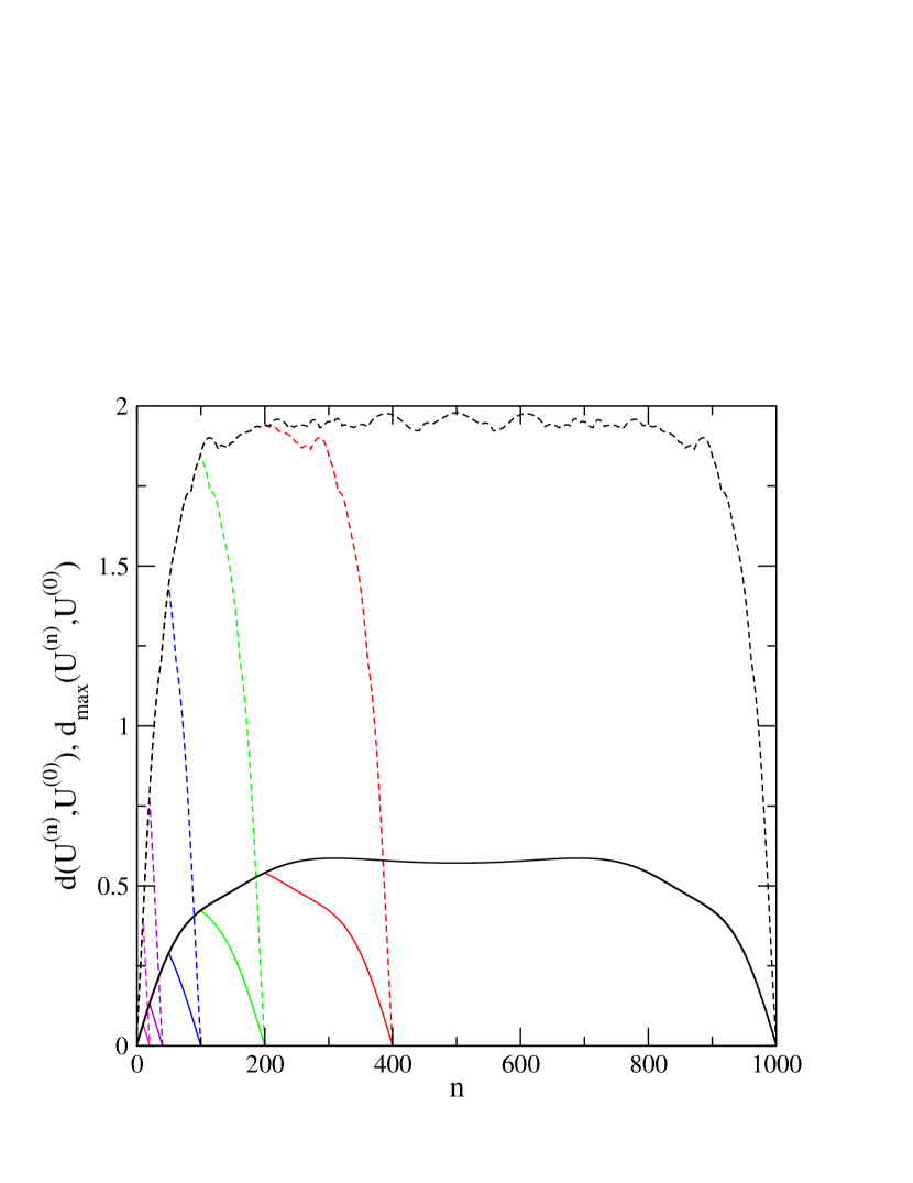
Figure 2: $d(U_{\mu}^{(n)},U^{(I)}_{\mu})$ and $d_{max}(U_{\mu}^{(n)},U^{(I)}_{\mu})$ in a trajectory of $m_{sea}=0.02$ on $16^{3}\times 32$. The total step numbers are 10, 20, 50, 100, 200, and 500. The solid curves are $d(U_{\mu}^{(n)},U^{(I)}_{\mu})$ while the dashed are $d_{max}(U_{\mu}^{(n)},U^{(I)}_{\mu})$.

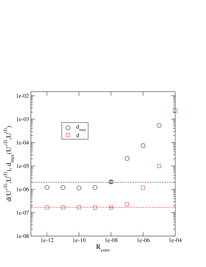
Figure 3: The breaking of reversible dynamics measured by $d(U^{{}^{\prime}(I)}_{\mu},U^{(I)}_{\mu})$ and $d_{max}(U^{{}^{\prime}(I)}_{\mu},U^{(I)}_{\mu})$ as a function of the CG convergence criteria, $R_{conv}$. The dotted lines are observed upper bound of deviations due to the reunitarization process. The error-bar at $R_{conv}$ = 1e-8 was obtained using five configurations.

where, for a generic matrix $M$, $\left\|M\right\|_{2}$ represents the $l_{2}$ norm Horn and Johnson (1986). These are plotted in Figure 2 for $N=20$, 40, 100, 200, 400, and 1000 using a starting configuration from the $m_{\rm sea}=0.02$ ensemble ($d(U^{(n)},U^{(I)})$ and $d_{max}(U^{(n)},U^{(I)})$ are relatively independent of the sea quark mass). The crucial issue is how small $R_{conv}$ must be so that the breaking of reversibility is negligible. In Figure 3, $d(U^{(N)},U^{(I)})$ and $d_{max}(U^{(N)},U^{(I)})$ are plotted as a function of $R_{conv}$, for a starting configuration in the $m_{\rm sea}=0.02$ ensemble and $N=102$; the value we use in our simulations. For $R_{conv}\geq 10^{-6}$ the MD is not reversible. $d(U^{(n)},U^{(I)}_{\mu})$ reaches the edge of floating point accuracy at $R_{conv}=10^{-7}$ but $d_{max}(U^{(n)}_{\mu},U^{(I)}_{\mu})$ is still resolved. For $R_{conv}\leq 10^{-8}$, both deviations are below single precision accuracy and comparable to the deviations due to reunitarization which are shown by the dotted lines in the graph. From these checks we choose $R_{conv}=10^{-8}$ as the CG convergence criterion in our simulation.

II.3 Multiple Time-scale Leapfrog evolution

In this section we discuss the multiple time-step leapfrog integration scheme of Sexton and Weingarten (1992). While this technique was not used in the main part of this work, a small study was performed to test its usefulness, the results of which will be included here as they are both encouraging and instructive.

In Sexton and Weingarten (1992) a procedure was outlined for constructing leapfrog integrators for which a different time-step size could be used for different parts of the molecular dynamics Hamiltonian. The parts of this Hamiltonian which produce the dominant contribution to the leap-frog integration discretization error may then be treated with a finer discretization than the remainder. In the case where the dominant contribution to the discretization error comes from the gauge piece of the Hamiltonian, for which the molecular dynamics force term is relatively inexpensive to compute, a large improvement in the efficiency of the algorithm is possible.

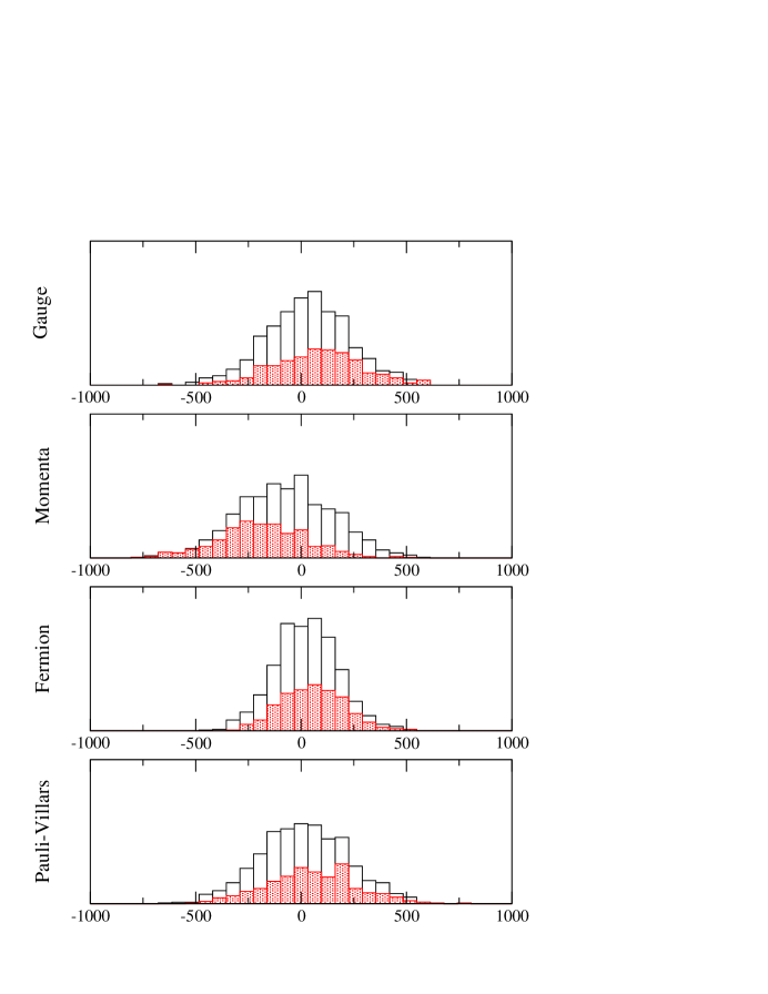
Figure 5: The individual contributions to the total change in the Hamiltonian from the various components of the Hamiltonian for the large step-size, old force term simulation described in Table 1. The shaded bars represent the trajectories which failed the accept/reject step, while the empty bars tally all trajectories.

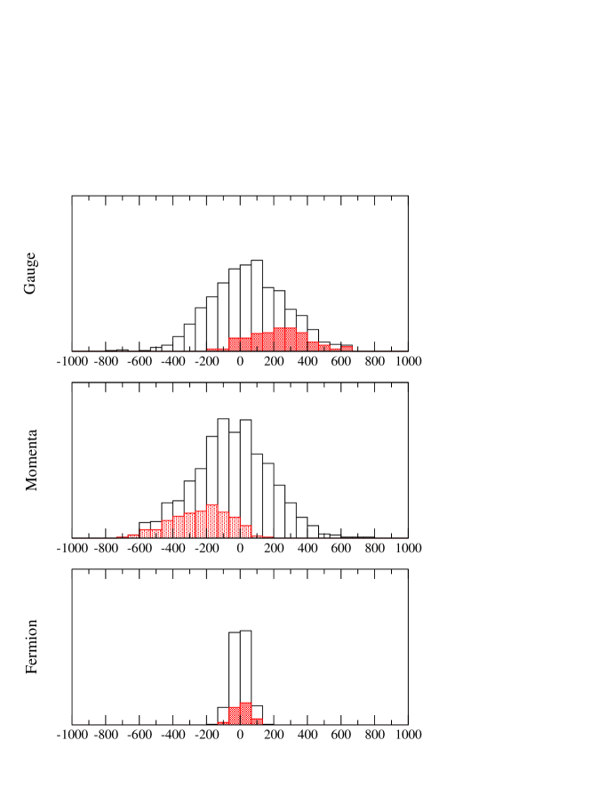
Figure 6: The individual contributions to the total change in the Hamiltonian from the various components of the Hamiltonian for the large step-size, new force term simulation described in Table 1. The shaded bars represent the trajectories which failed the accept/reject step, while the empty bars tally all trajectories. Note that the magnitude of the differences is dominated by the gauge and momentum parts of the Hamiltonian, and the noticeable trend that trajectories for which the change in the gauge part of the Hamiltonian is positive are more likely to be rejected.

For the standard actions this does not seem to be the case. However, there is some evidence that when using the modified force term described in Section II.1 the dominant errors are coming from the gauge part of the action. Figures 5 and 6 contrast the individual contributions of the gauge, momentum, fermion and Pauli-Villars terms to the total change in the Hamiltonian over a trajectory for the small volume, large step size runs tabulated in Table 1. As can be seen, for the old force term this change is approximately the same size for all contributions, while for new force term the gauge and momenta contributions are much larger than the (combined) fermion contribution. There is also a noticeable skew in the distributions for the gauge and momenta pieces of the Hamiltonian, with a positive change in the gauge Hamiltonian being rejected much more often than a negative change.

To test if the discretization error for the new force term is, indeed, dominated by the contributions from the gauge and momenta pieces of the Hamiltonian, we have performed a trial of the multiple gauge-step leapfrog integrator over 45 trajectories, starting from trajectory 1505 of the $m_{\rm sea}=0.04$ evolution. Over this range the standard algorithm had an acceptance of 56%. Performing two gauge integration steps for every fermion integration step the acceptance moved up to 91%, confirming the gauge momenta pieces are the dominant cause of the discretization error. While we would like to exploit this fact by using a large fermion step-size combined with a small gauge step-size, we have found that in the few tests that we have undertaken the performance of the chronological invertor degrades as the fermion step-size increases by an amount that almost completely offsets the fewer number of inversions needed. However, this is an approach worthy of a more extended study, and even if it does not allow the move to larger fermion step-sizes, the gain in acceptance we have observed is appreciable.

III Simulation Details

As mentioned previously, our simulations have been made using the standard domain wall Dirac operator Furman and Shamir (1995), combined with the Paulli-Villars field with the action introduced in Vranas (1998). For each of our three dynamical ensembles we employ two dynamical flavors, with $L_{s}=12$ and $M_{5}=1.8$ (we use the notation and conventions introduced in Blum et al. (2004) for the domain wall fermion action), on lattices of size $16^{3}\times 32$. The fermion boundary conditions are periodic in the spatial directions and anti-periodic in the time direction. These ensembles have bare quark masses of $0.02$, $0.03$ and $0.04$. The basic HMC parameters are tabulated in Table 2; all Dirac matrix inversions were performed using the conjugate gradient algorithm with a stopping condition of $10^{-8}$.

We use the DBW2 gauge action Takaishi (1996) with $\beta=0.80$, the same action we have used in previous quenched studies Aoki et al. (2004a, c). This action approximates the renormalization group trajectory by using the standard plaquette, $P_{1\times 1}$, and a $1\times 2$ rectangular plaquette, $P_{1\times 2}$:

$$S_{g} = -\frac{\beta}{3}\,\left(\sum_{x}\,\left(1-8c_{1}\right)\,{\rm Tr}\,P_{1\times 1}+c_{1}\,{\rm Tr\,P_{1\times 2}}\right)\,.$$ (14)

This form was originally suggested by Iwasaki Iwasaki (1983a, b); Iwasaki and Yoshie (1984), who, using a perturbative approach, estimated a value of $c_{1}=-0.331$. In de Forcrand et al. (2000) a non-perturbative estimate, of $c_{1}=-1.4069$, was made in the quenched approximation. While we are working with dynamical fermions, this is the value we use; our intent being to exploit the improvement in the chiral properties of domain wall fermions that this gauge action provides Aoki et al. (2004a), rather than to be as close as possible to the renormalized trajectory. Of course, it is possible that the effects of the determinant will negate any such improvement. This issue is discussed further in section VI.

IV Thermalization and Auto-correlations

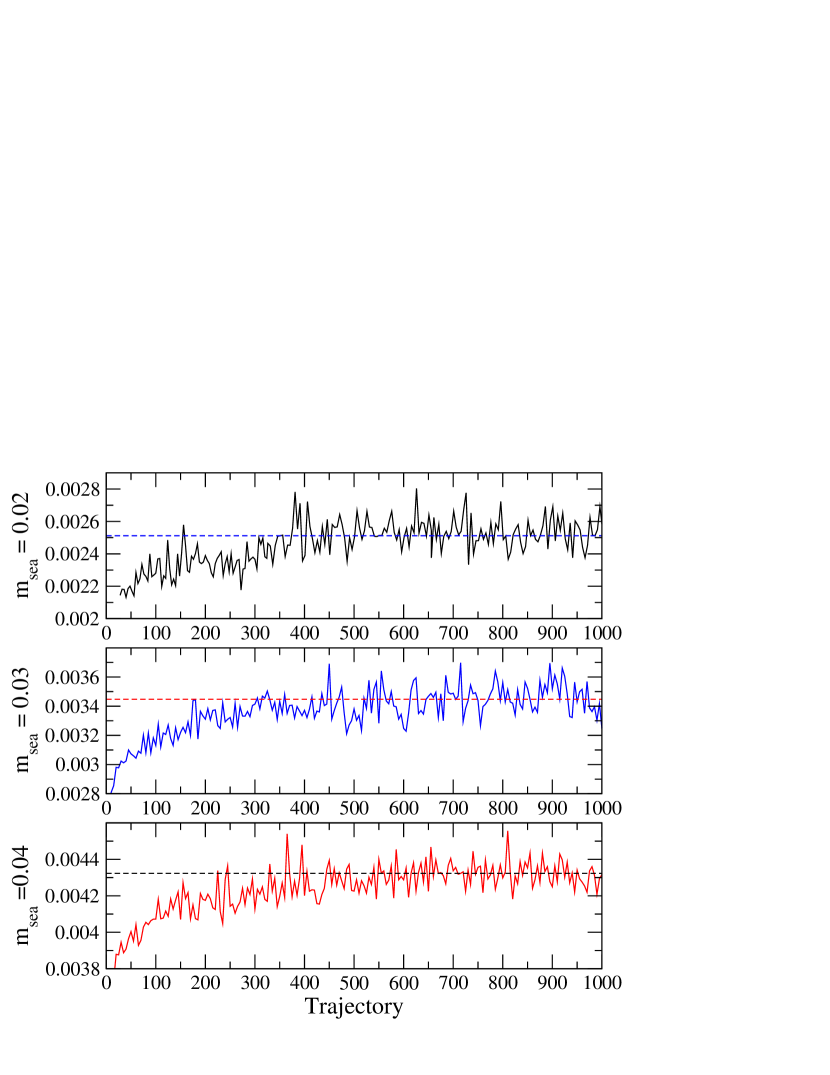
Figure 7: The history of $\overline{q}q$ ($m_{\rm val}=m_{\rm dyn}$), up to trajectory 1000, for all evolutions. The average from trajectory 3000 onwards is shown as a dashed horizontal line.

In this section we discuss the related issues of thermalization and auto-correlations for quantities calculated on our ensembles. Each evolution started from an ordered lattice, running for $O(10)$ trajectories without the accept/reject step applied, and leaving $O(600)$ trajectories for the lattice to thermalize. The precise numbers for each evolution are given in Table 4. As a check of the number of trajectories needed to thermalize the configurations we have calculated chiral condensate $\langle\overline{q}{q}\rangle(m_{\rm val}=m_{\rm sea})$ on every trajectory, using a single hit of a random source. Figure 7 shows this, together with the average value for trajectory 3000 and above, which agree well with each other by the 600th trajectory.

For the results presented later in this work we use 94 configurations from each ensemble, separated by 50 HMC trajectories. For the $m_{\rm sea}=0.02$ and $m_{\rm sea}=0.03$ ensembles these configurations are taken sequentially from the thermalization point given in Table 4. For the $m_{\rm sea}=0.04$ evolution we leave a gap of 250 trajectories, starting from trajectory 1775, due to a hardware error on trajectory 1772 that was not detected until after the entire evolution was finished. The trajectory passed the accept/reject step, and no effect was seen in any of the physical observables that we have calculated; nevertheless, to be cautious, we have allowed this gap of 250 trajectories for the evolution to re-thermalize. Table 5 gives the results for the bare lattice values of the chiral condensate (for $m_{\rm val}=m_{\rm sea}$), and the $r\times t$ on-axis Wilson loop, $\langle W(r,t)\rangle$, with $(r,t)=\{(1,1),(1,2),(2,2),(3,3)\}$ for these sets of configurations. While we do not use these values in the rest of this work, we include them here as they may be of utility for others trying to work at this set of parameters.

To test this spacing of 50 trajectories we have calculated the auto-correlation function, defined for some observable, ${\cal O}(t)$ (here $t$ labels the trajectory, and runs from 1 to $N_{data}$), as

$$\rho(t) = {\frac{1}{N_{data}-t}}\sum_{t^{\prime}=1}^{N_{data}-t}\left({\cal O}(t^{\prime})-\bar{\cal O}\right)\left({\cal O}(t^{\prime}+t)-\bar{\cal O}\right)~{}~{},$$ (15)

$$\bar{\cal O} = {\frac{1}{N_{data}}}\sum_{t^{\prime}=1}^{N_{data}}{\cal O}(t^{\prime})\ ,$$ (16)

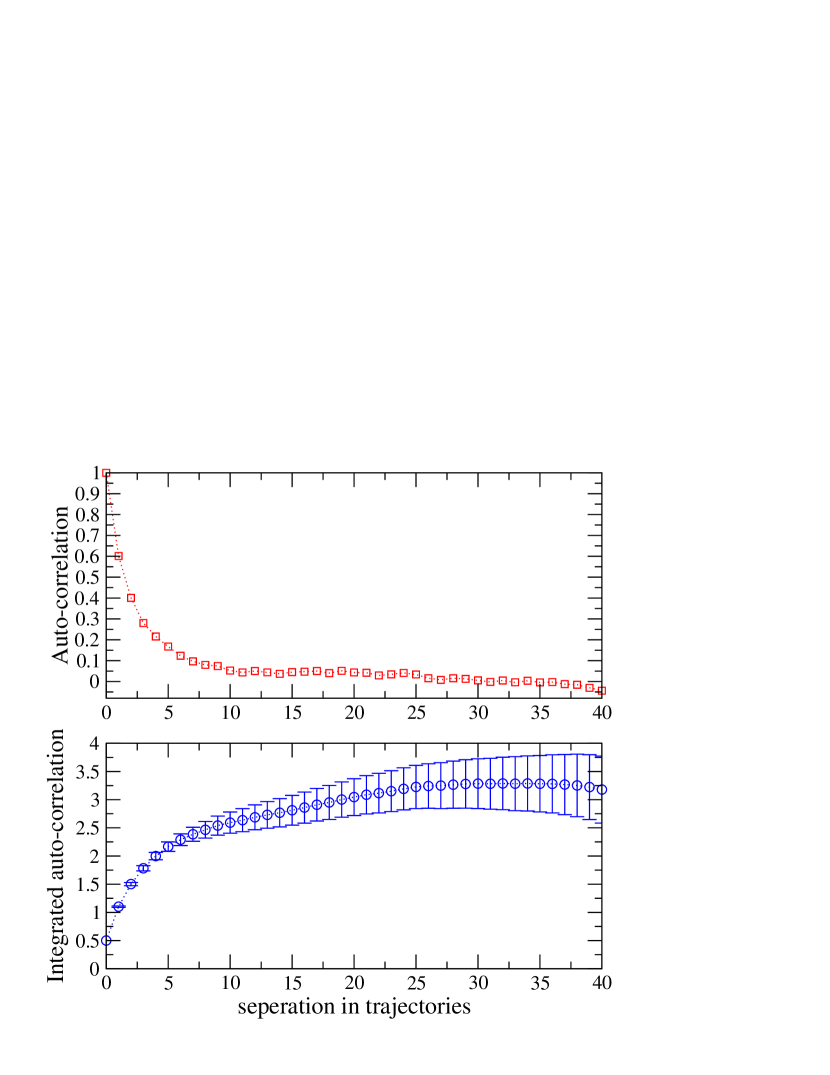
Figure 8: Plaquette auto-correlation function and integrated auto-correlation length for the $m_{\rm sea}=0.02$ ensemble.

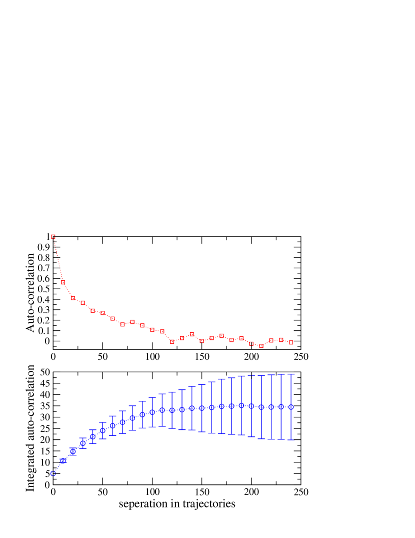
Figure 9: Auto-correlation function and integrated auto-correlation length for timeslice 12 of the correlation function of the time component of the local axial vector current on the $m_{\rm sea}=0.02$ ensemble.

on the $m_{\rm sea}=0.02$ ensemble for the plaquette and the correlation function of the time component of the local axial vector current at time slice 12. The former was measured every trajectory, while the latter was calculated every 10 trajectories using a Coulomb gauge-fixed box source of size 10 and a point sink. Figures 8 and 9 show both the normalized auto-correlation function, $\rho(t)/\rho(0)$, and the integrated auto-correlation length,

$$\tau_{int}(t_{max})={\frac{1}{2}}+\frac{1}{\rho(0)}\sum_{t=1}^{t_{max}}\rho(t)\ ,$$ (17)

for these two quantities, versus the separation in trajectories and the maximum separation over which correlations were calculated, $t_{max}$, respectively. The quoted error on the integrated auto-correlation length is calculated using a jackknife procedure: as is standard, each jackknife sample is constructed by removing a contiguous group of data-points, covering $N_{block}$ trajectories, from the available data. On the $j^{th}$ jackknife sample ($j\in[0,N_{data}/N_{block})$) we construct an estimate of the auto-correlation function,

$$\rho_{j}(t) = \frac{1}{N_{sum}}\left(\sum_{t^{\prime}=1}^{jN_{block}-t}\left({\cal O}(t^{\prime})-\bar{\cal O}_{j}\right)\left({\cal O}(t^{\prime}+t)-\bar{\cal O}_{j}\right)\right.$$

$$+ \left.\sum_{t^{\prime}=(j+1)N_{block}+1}^{N_{data}-t}\left({\cal O}(t^{\prime})-\bar{\cal O}_{j}\right)\left({\cal O}(t^{\prime}+t)-\bar{\cal O}_{j}\right)\right)\ ,$$

$$\bar{\cal O}_{j} = {\frac{1}{N_{data}-N_{block}}}\left(\sum_{t^{\prime}=1}^{jN_{block}}{\cal O}(t^{\prime})+\sum_{t^{\prime}=(j+1)N_{block}+1}^{N_{data}}{\cal O}(t^{\prime})\right)$$ (19)

where $N_{sum}$ is the total number if terms in the two summations; this is not simply $N_{data}-N_{block}-t$, as if $t$ is greater than or equal to $jN_{block}$ or $N_{data}-(j+1)N_{block}$ we must drop the first or last summation, respectively, in Equation IV. Estimates of the integrated auto-correlation length on every jackknife sample are constructed from Equation 17 and used to calculate the error in the standard fashion. Ideally, we would like to work in the regime such that $N_{block}\gg t_{max},\tau_{int}$ for a value of $N_{block}$ which leads to an appreciable number of jackknife samples. Here we use $N_{block}=100$. This leads to acceptable number of jackknife samples ($\sim 50$), but may be too short for a solid estimation of the error for the axial-axial data. As can be seen from Figures 8 and 9, the integrated auto-correlation length plateaus at $\approx 3$ for the plaquette and $\approx 35$ for the axial-axial correlator. While these values would suggest that the auto-correlations may be under control for our configurations, caution should be taken both because their extraction is insensitive to correlations longer than $O(100)$ trajectories, and because the auto-correlation length depends on the quantity.

An important example of a quantity which displays correlations over the scale of many hundreds of trajectories is the topological charge. To calculate the topological charge the lattices are first smoothed by applying 20 steps of APE smearing with a coefficient of 0.45; then the topological charge is measured using a discretization of the operator

$$Q_{\rm top}=\frac{1}{32\pi^{2}}\epsilon_{ijkl}\mathrm{Tr}\left[F_{ij}F_{kl}\right]\,,$$ (20)

which is based upon two definitions of the lattice field strength tensor, $F_{\mu\nu}$: that using the clover leaf pattern for the simple ($1\times 1$) plaquette,

$$F^{C}_{\mu\nu}=-\frac{i}{4}\;{\rm An}\left(\raisebox{-11.38092pt}{ \begin{picture}(2.7,2.3)(-1.15,-1.15)\put(-1.15,-1.15){\begin{picture}(1.15,1.15)(-0.575,-0.575) \put(-0.5,-0.5){\line(1,0){1.0}} \put(0.5,-0.5){\line(0,1){1.0}} \put(0.5,0.5){\line(-1,0){1.0}} \put(-0.5,0.5){\line(0,-1){1.0}} \end{picture}}\put(0.0,0.0){\begin{picture}(1.15,1.15)(-0.575,-0.575) \put(-0.5,-0.5){\line(1,0){1.0}} \put(0.5,-0.5){\line(0,1){1.0}} \put(0.5,0.5){\line(-1,0){1.0}} \put(-0.5,0.5){\line(0,-1){1.0}} \end{picture}} \put(-1.15,0.0){\begin{picture}(1.15,1.15)(-0.575,-0.575) \put(-0.5,-0.5){\line(1,0){1.0}} \put(0.5,-0.5){\line(0,1){1.0}} \put(0.5,0.5){\line(-1,0){1.0}} \put(-0.5,0.5){\line(0,-1){1.0}} \end{picture}}\put(0.0,-1.15){\begin{picture}(1.15,1.15)(-0.575,-0.575) \put(-0.5,-0.5){\line(1,0){1.0}} \put(0.5,-0.5){\line(0,1){1.0}} \put(0.5,0.5){\line(-1,0){1.0}} \put(-0.5,0.5){\line(0,-1){1.0}} \end{picture}} \put(0.0,0.0){\circle*{0.3}} \end{picture}}\right)\,,$$ (21)

and the analogous quantity for the $2\times 1$ rectangle,

$$F^{R}_{\mu\nu}=-\frac{i}{16}\;{\rm An}\left(\raisebox{-11.38092pt}{ \begin{picture}(2.6,2.6)(-1.55,-1.15)\put(-1.15,0.0){\begin{picture}(1.15,1.15)(-0.575,-0.575) \put(-1.0,-0.5){\line(1,0){2.0}} \put(-1.0,0.5){\line(1,0){2.0}} \put(-1.0,-0.5){\line(0,1){1.0}} \put(1.0,-0.5){\line(0,1){1.0}} \end{picture}}\put(1.0,0.0){\begin{picture}(1.15,1.15)(-0.575,-0.575) \put(-1.0,-0.5){\line(1,0){2.0}} \put(-1.0,0.5){\line(1,0){2.0}} \put(-1.0,-0.5){\line(0,1){1.0}} \put(1.0,-0.5){\line(0,1){1.0}} \end{picture}} \put(-1.15,-1.15){\begin{picture}(1.15,1.15)(-0.575,-0.575) \put(-1.0,-0.5){\line(1,0){2.0}} \put(-1.0,0.5){\line(1,0){2.0}} \put(-1.0,-0.5){\line(0,1){1.0}} \put(1.0,-0.5){\line(0,1){1.0}} \end{picture}}\put(1.0,-1.15){\begin{picture}(1.15,1.15)(-0.575,-0.575) \put(-1.0,-0.5){\line(1,0){2.0}} \put(-1.0,0.5){\line(1,0){2.0}} \put(-1.0,-0.5){\line(0,1){1.0}} \put(1.0,-0.5){\line(0,1){1.0}} \end{picture}} \put(0.5,0.0){\circle*{0.3}} \end{picture}}\hskip 22.76228pt+\ \ \raisebox{-11.38092pt}{ \begin{picture}(2.6,2.6)(-1.55,-1.55)\put(-2.15,0.0){\begin{picture}(1.15,1.15)(-0.575,-0.575) \put(-0.5,-1.0){\line(1,0){1.0}} \put(-0.5,1.0){\line(1,0){1.0}} \put(-0.5,-1.0){\line(0,1){2.0}} \put(0.5,-1.0){\line(0,1){2.0}} \end{picture}}\put(-1.0,0.0){\begin{picture}(1.15,1.15)(-0.575,-0.575) \put(-0.5,-1.0){\line(1,0){1.0}} \put(-0.5,1.0){\line(1,0){1.0}} \put(-0.5,-1.0){\line(0,1){2.0}} \put(0.5,-1.0){\line(0,1){2.0}} \end{picture}} \put(-2.15,-2.15){\begin{picture}(1.15,1.15)(-0.575,-0.575) \put(-0.5,-1.0){\line(1,0){1.0}} \put(-0.5,1.0){\line(1,0){1.0}} \put(-0.5,-1.0){\line(0,1){2.0}} \put(0.5,-1.0){\line(0,1){2.0}} \end{picture}}\put(-1.0,-2.15){\begin{picture}(1.15,1.15)(-0.575,-0.575) \put(-0.5,-1.0){\line(1,0){1.0}} \put(-0.5,1.0){\line(1,0){1.0}} \put(-0.5,-1.0){\line(0,1){2.0}} \put(0.5,-1.0){\line(0,1){2.0}} \end{picture}} \put(-1.0,-0.5){\circle*{0.3}} \end{picture}}\right)\,,$$ (22)

where

$${\rm An}\left(M\right)=\frac{1}{2}\left(M-M^{\dagger}\right)\,.$$ (23)

While equations 21 and 22 may simply be substituted into equation 20 to obtain discretized expressions for the topological charge (which we denote $Q^{C}$ and $Q^{R}$, respectively), they may also be combined such that the $O(a^{2})$ errors cancel between the two definitions. This gives the improved topological charge operator Ali Khan et al. (2001c):

$$Q^{\rm imp}_{2}=\frac{5}{3}Q^{C}-\frac{2}{3}Q^{R}\,.$$ (24)

We may also construct a definition built up from a classically $O(a^{2})$ improved field strength tensor Bilson-Thompson et al. (2003):

$$Q^{\rm imp}_{4}=\frac{25}{9}Q^{C}-\frac{20}{9}\frac{1}{32\pi^{2}}\epsilon_{ijkl}\mathrm{Tr}\left[F^{C}_{ij}F^{R}_{kl}\right]+\frac{4}{9}Q^{R}\,,$$ (25)

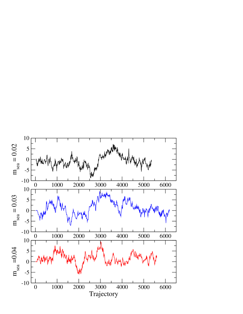
Figure 10: Topological charge history for all the ensembles. Note the correlations of the scale of many hundreds of HMC trajectories.

which is also $O(a^{2})$ improved, but which has different $O(a^{4})$ errors. We use this last operator to quote our values of the topological charge, although there would be little difference if we had decided to use the operator of Equation 24: for the 2565 topological charge measurements made on our dynamical ensembles, we observed only 3 cases in which these two discretizations differed when rounded to the the nearest integer. We have also compared our values to those calculated using the topological charge operator of DeGrand et al. (1998): for a test over 418 measurements from the $m_{sea}=0.03$ evolution we found $90\%$ agreement on the nearest integer, with the largest absolute difference being 0.76. Figure 10 shows these topological charge values versus trajectory for all of the ensembles. Note the correlations over many hundreds of HMC trajectories. Although the DBW2 action suppresses topology changing configurations (this is the reason for its improved chiral properties in conjunction with domain wall fermions)Aoki et al. (2004a), considering the relatively large level of explicit chiral symmetry breaking observed in our simulations (see sections V and VI), we believe the long correlation length observed here is due mainly to the small trajectory length HMC algorithm which is known to move slowly between topological sectorsIlgenfritz et al. (2000).

V Physical Results

V.1 hadron spectrum and decay constants

In this work hadron masses are extracted using standard covariant fits (see, e.g. Toussaint (1989)) of two-point correlation functions at relatively large Euclidean time interval from a single meson or baryon source located at $t=0$, so that only a single exponential corresponding to the ground state is fit in each case. The source is either a Coulomb gauge-fixed wall source or a plain wall source. The latter corresponds to averaging over a point source on a time-slice after averaging over the gauge field ensemble. We use only point sinks. The wall sources generally have better overlap with the ground states in which we are most interested, and therefore lead to more accurate determination of the particle masses. However, the decay constants are more easily obtained from the point source matrix elements. In the case of the point source, we also computed the correlation functions using a source located at $t=16$, i.e. the maximum distance from the original source on our periodic lattice, in order to improve our statistics. We consider zero momentum states only. All quoted statistical errors are estimated by fitting the correlation functions under a standard single-elimination jackknife procedure.

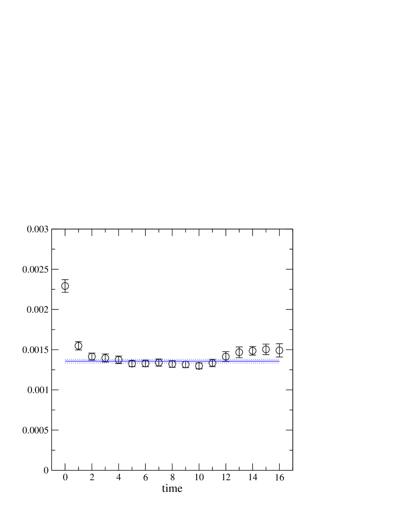
Figure 11: The residual mass plateau plot for $m_{sea}=m_{val}=0.02$. The error-weighted average between timeslices 4 and 16 is shown as a horizontal line.

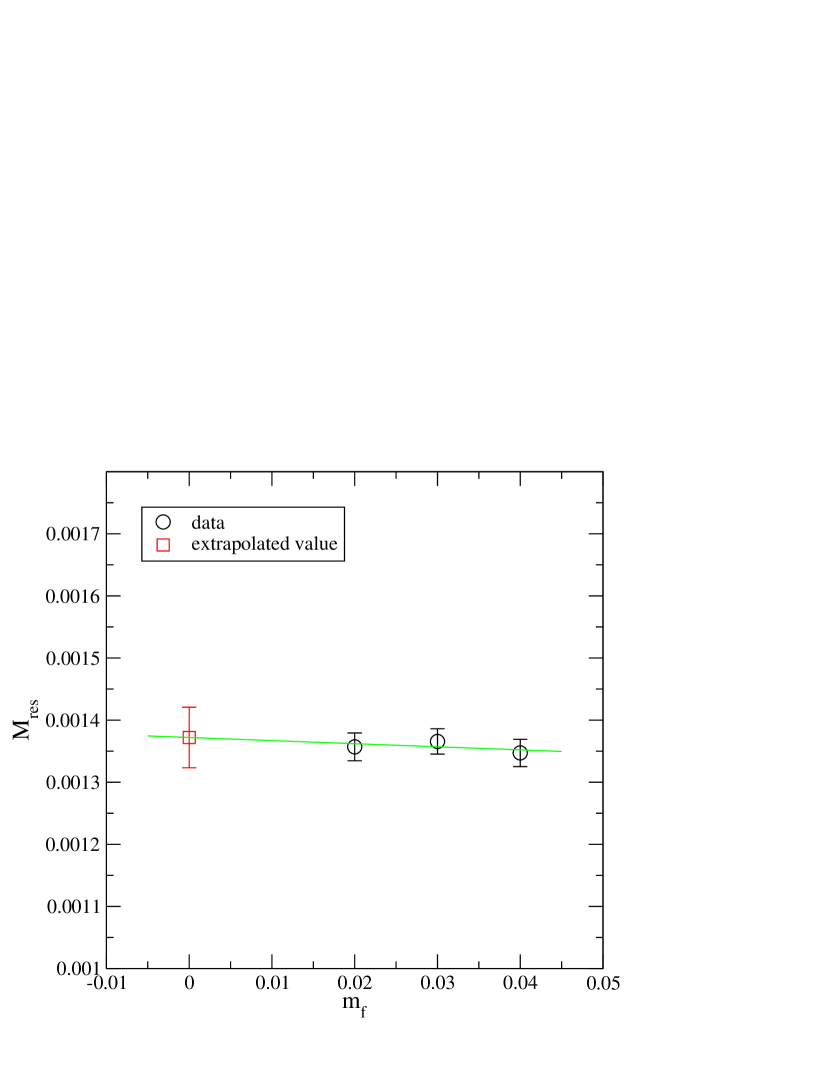
Figure 12: The residual mass extrapolated to $m_{sea}=m_{val}=0.0$.

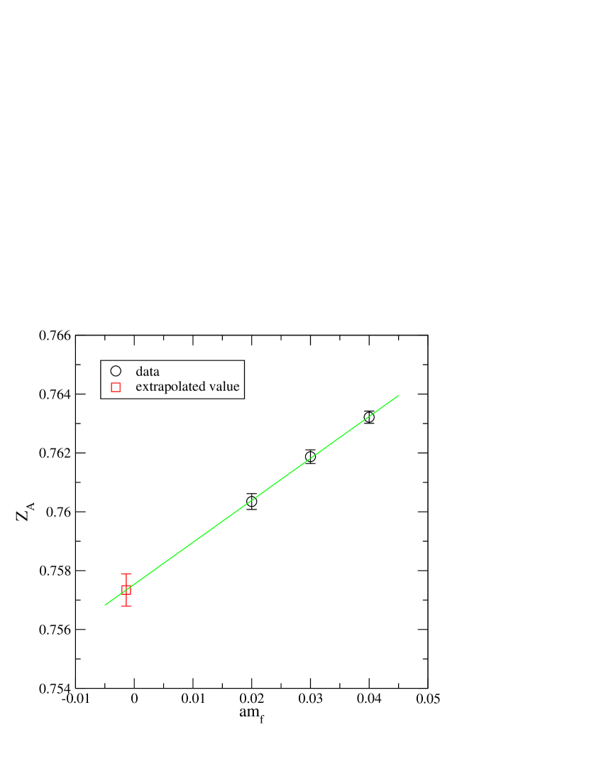
Figure 13: The renormalisation factor for the local, non-singlet, axial current. This is defined in the chiral limit. Here we show the data at finite mass for the fully dynamical points together with the results of a linear extrapolation to the chiral limit.

We begin with the calculation of the residual mass, $m_{\rm res}$, in order to define the chiral limit, $m_{f}=-m_{\rm res}$. $m_{\rm res}$ is the additive renormalization of the quark mass caused by mixing between the left and right handed fermions localized on opposite boundaries of the fifth dimension and is defined from the explicit chiral symmetry breaking term in the axial Ward-Takahashi identity for domain wall fermionsBlum et al. (2004). We refer the reader to Blum et al. (2004); Aoki et al. (2004a) for details of the method to calculate $m_{\rm res}$. In Figure 11 the effective residual mass, $R(t)$, for $m_{\rm sea}=m_{\rm val}=0.02$ is shown for each time slice (because the correlator is periodic, we fold the correlation functions about the mid-point of the lattice in the time direction which is why our plots range from $t=0$ to 16). It falls by about a factor of 2 over the first couple of times slices and then remains constant. This non-local effect of the extra dimension of domain wall fermions is well known Aoki et al. (2004a); Golterman and Shamir (2003). Taking the error-weighted average over time slices 4 through 16 and linearly extrapolating the $m_{\rm sea}=m_{\rm val}$ points to $m_{f}=0$, we find $am_{\rm res}=0.001372(49)$ (see Figure 12). We also use the axial Ward-Takahashi identity and the partially conserved axial-vector current to extract the renormalization factor $Z_{A}$ appearing in Eq. 32Blum et al. (2004). We find $Z_{A}=0.75734(55)$, defined in the chiral limit, and extracted from a linear fit to the mass dependence of the fully dynamical points (see Figure 13).

Next, we turn to the vector meson mass. In principle, the vector particle can decay hadronically into two pseudo-scalars since vacuum sea quark effects are included in this two flavor simulation. However, in the regime we are working the sea quarks are still relatively heavy, and, taking into account that two pions must have relative orbital angular momentum $L=1$ for the decay to be allowed, it is easy to note that our vector mass is always below the threshold for this decay. Thus the two pion states, while present in this channel, represent excited states.

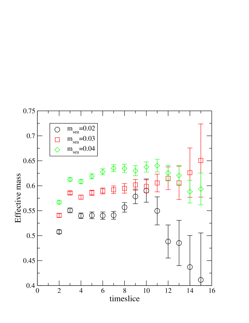
Figure 14: The effective mass in the vector channel for $m_{sea}=m_{val}$.

Figure 14 displays the effective mass in the vector channel, $m_{\rm sea}=m_{\rm val}$, averaged over all three spatial polarizations. Tables 6 -8 give the fitted masses from the wall-point correlation functions for all combinations of sea and valence quark masses for a set of time slice ranges chosen based on the effective mass plateaus shown in Figure 14. The masses are extracted from a fit to

$$\lim_{t\to\infty}G(t) = A\left(e^{-m\,t}+e^{-m\,(N_{t}-t)}\right)$$ (26)

$$= {2A}e^{-m(N_{t}/2)}\cosh{(m\,(N_{t}/2-t))}.$$ (27)

The mass plateaus are rather poor, especially for $m_{\rm sea}=0.02$, which is reflected in the values of $\chi^{2}$ for the fits. Additional statistics are desirable, though we note our trajectory lengths are already quite long for dynamical fermion simulations ($\sim 5000$). Table 9 shows the results of performing two fits to the data in Tables 6-8: a linear fit to the fully dynamical, $m_{\rm sea}=m_{\rm val}$, points,

$$M_{vector}=a+b(m_{sea}+m_{res})\,,$$ (28)

and a partially quenched fit to all the data,

$$M_{vector}=a+b(m_{sea}+m_{res})+c(m_{val}+m_{res})\,.$$ (29)

As can be seen from the consistancy of these two fits, the linear ansatz works well for this data. Considering the small mass range available, we do not attempt more sophisticated fits. The linear extrapolation of the three (uncorrelated) points $m_{\rm sea}=m_{\rm val}$ to $\bar{m}=(m_{u}+m_{d})/2$ (later, when we discuss the pseudo-scalar meson, we will see how $\bar{m}$ is determined) yields the value of the vector meson mass corresponding to the physical $\rho$ meson. From $M_{\rho}=770{\rm MeV}$ we find

$$a^{-1}_{\rho}=1.691(53)\,{\rm GeV}.$$ (30)

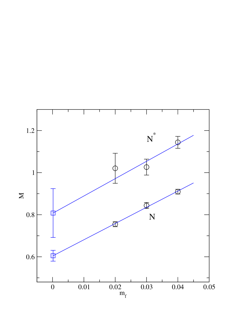
Figure 23: The masses of nucleon and its parity partner for the dynamical points ($m_{f}=m_{\rm sea}=m_{\rm val}$). The solid line is a simple linear fit. Square symbols show the extrapolated results at $m_{f}=\bar{m}$.

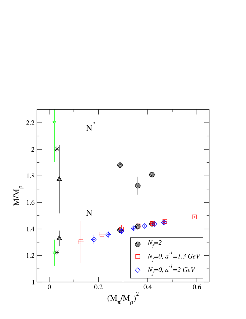
Figure 24: APE plot of nucleon and its parity partner. Filled symbols show the dynamical DWF results, while open symbols show the quenched DWF results Aoki et al. (2004a) with $a^{-1}\simeq 1.3$ GeV (squares) and $a^{-1}\simeq 2$ GeV (diamonds). The upper and lower triangles are dynamical DWF results at the physical light quark mass ($\bar{m}$) with diagonal and two stage chiral extrapolations from Table 13, Stars indicate experimental values, $N(939)$ and $N^{*}(1535)$.

A similar analysis has been carried through for the nucleon mass. This is calculated from Coulomb gauge-fixed wall-point two point functions of the interpolating field, $J_{N}=\epsilon^{ijk}(u^{iT}C\gamma_{5}d^{j})u^{k}$, using a positive parity projection. The results of a fit to a single exponential ($Ae^{-mt}$) are shown in Table 10. Taking the negative parity projection we may also extract the mass of the $N^{*}$, the parity partner of the nucleon, the results for which are tabulated in Table 11. Figure 23 shows both these quantities for the dynamical, $m_{\rm sea}=m_{\rm val}$, points. In Figure 24 we show the APE plot ($M_{I}/M_{\rho}$ vs. $(M_{\pi}/M_{\rho})^{2}$ where $M_{I}$ is represents the mass of the $N$ or $N^{*}$), together with the results from quenched DWF with DBW2 gauge action Aoki et al. (2004a) for the nucleon. We note that the dynamical and the quenched values are in good agreement. Of course, in a comparison between the nucleon and rho masses, we must bear in mind that the rho is stable for all values of the quark masses studied here, which introduces a systematic error that could easily be 10% or more in the ratio $m_{N}/m_{\rho}$. However, we are encouraged to think that our error in $m_{\rho}$ may be smaller than this, since the value of the lattice spacing determined from the rho mass agrees quite closely with that implied by our calculation of $f_{\pi}$ and of the Sommer scale, $r_{0}$, as discussed later in this section and in Section V.2, respectively.

In Figures 23 and 24, we show an extrapolation to the physical point, $m_{f}=\bar{m}$. To perform this extrapolation we have used a linear ansatz for the quark mass dependence of the nucleon. The extrapolated values shown in the figures are taken from a fit to just the dynamical points, the results of which are given in Table12. As can be seen, the nucleon mass is two standard deviations (9%) larger than experiment. Note that our spatial lattice size, $L\simeq 1.9$ fm is not small enough that we would expect to see significant finite volume effects in our data for the quark masses we are using; $LM_{\pi}\simeq 4.7$ for our lightest mass. Systematic numerical studies Orth et al. (2004); Orth (2004); Ali Khan et al. (2004), as well as theoretical calculations Beane (2004a), on the finite volume effects in the nucleon mass with two flavor Wilson fermions indicate a few percent finite volume mass shift with similar parameters to our lightest point. However, as the $\rho$ mass receives similar finite volume effectOrth et al. (2004); Orth (2004), the ratio at the physical limit can shift as little as $\mathrel{\hbox to0.0pt{\raise 2.20013pt\hbox{$<$}\hss}{\lower 2.20013pt\hbox{$\sim$}}}1\%$. Assuming that holds also for DWF, finite volume effect may be responsible for a minor part of the discrepancy. In addition, the systematic error associated with the linear fit is at least of the scale of this discrepancy. This can be seen by comparing the diagonal extrapolation and two stage linear extrapolation, where the valence limit $m_{\rm val}\to\bar{m}$ is taken first with fixed $m_{\rm sea}$, then dynamical extrapolation $m_{\rm sea}\to\bar{m}$ is performed. The result is shown in Table 12, Table 13, and in Figure 24 (triangle down). The difference between the two extrapolations indicates inapplicability of the linear ansatz. This ansatz clearly does not properly account for observed mass dependence of the nucleon. However, the statistical accuracy on the nucleon mass needs to be improved before more appropriate fits can be used Jenkins (1992); Leinweber et al. (2000); Bernard et al. (2004); Procura et al. (2004); Beane (2004b).

The physical $N^{*}$ mass is studied similarly. The diagonal and two stage extrapolations yield different results, but both are consistent with experiment to within one standard deviation (10%) below and above. We note that the $M_{N^{*}}$ at the lightest simulated point might suffer from the threshold effect, since $M_{N}+M_{\pi}=1.045(12)$ and $M_{N^{*}}=1.021(71)$. However the large statistical uncertainty prevents us from discussing further on this point.

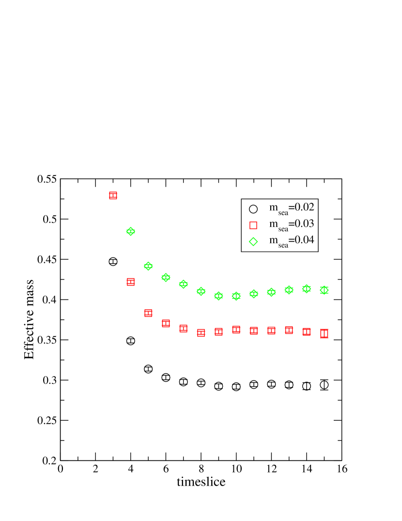
Figure 16: The effective mass in the pseudo-scalar channel for $m_{sea}=m_{val}=0.02$ (circles), 0.03 (squares), and 0.04 (triangles). Here we use the point-point Kuramashi-source correlation function. Similar results hold for $m_{sea}\neq m_{val}$.

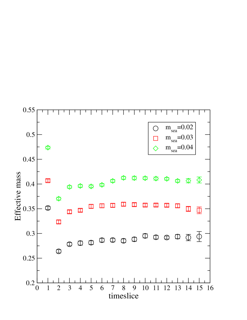
Figure 17: The effective mass in the pseudo-scalar channel for $m_{sea}=m_{val}=0.02$ (circles), 0.03 (squares), and 0.04 (triangles). Here we use a Coulomb-gauge-fixed wall sourcewith a point sink. Similar results hold for $m_{sea}\neq m_{val}$.

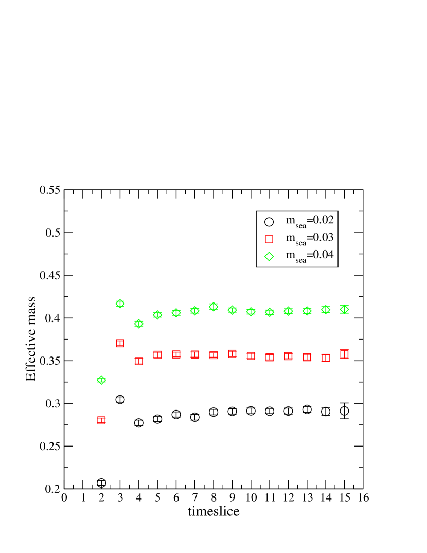
Figure 18: The effective mass in the axial-vector channel for $m_{sea}=m_{val}=0.02$ (circles), 0.03 (squares), and 0.04 (diamonds). Here we use a Coulomb-gauge-fixed wall sourcewith a point sink. Similar results hold for $m_{sea}\neq m_{val}$.

The analysis of the pseudo-scalar mesons will be somewhat more involved since partially-quenched chiral perturbation theory is at our disposal, and there are two channels, pseudo-scalar and the axial vector, which couple to the physical pion and kaon states. Figures 16-18 show the pseudo-scalar meson effective mass computed from the point-point and wall-point correlation functions. In each case we show $m_{\rm sea}=m_{\rm val}$; however the cases where $m_{\rm sea}\neq m_{\rm val}$ are similar. As expected, the point-point correlators exhibit plateaus that emerge at later times compared to the wall-point ones. As the quark mass increases, even the latter plateau emerges (from below) at rather late times. The statistical errors for the point-point axial-vector case are somewhat larger than for the others, especially at smaller valence quark mass. Based on the above plateaus we fit the correlation functions from $t_{min}=9$ to $t_{max}=16$. The results do not change by more than one standard deviation when $t_{min}$ is changed by two units in either direction, provided $\chi^{2}$/dof remains acceptable which was almost always the case. Results for all quark mass combinations are summarized in Tables 14-17. Fitted meson masses among these four methods are mostly consistent within one (statistical) standard deviation, except for the lightest point ($m_{\rm sea}=0.02$, $m_{\rm val}=0.01$) where the mass in the point-point pseudo-scalar channel is almost two standard deviations higher than the rest. This may indicate that our statistical errors are underestimated due to the limited length in simulation time of our evolution ($\sim 5000$ trajectories).

The pseudo-scalar decay constant $f_{PS}$ is obtained from the point-point correlation function, either directly (axial-vector), or through the Ward-Takahashi identity (pseudo-scalar) Blum et al. (2004); Aoki et al. (2004a). When using a point source, $A$ in Eq. 26 is proportional to the square of the decay constant. Specializing to the pseudo-scalar,

$$A = \frac{|\langle 0|\chi|PS\rangle|^{2}}{2M_{PS}},$$ (31)

where $\chi=\bar{\psi}\gamma_{\mu}\gamma_{5}\psi$ for the axial vector and $\bar{\psi}\gamma_{5}\psi$ for the pseudo scalar, and $M_{PS}$ is the pseudo-scalar mass. We have for the lattice matrix elements

$$\langle 0|\bar{\psi}\gamma_{4}\gamma_{5}\psi|PS\rangle = f^{lat}_{PS}\,M_{PS}=\frac{f_{PS}}{Z_{A}}\,M_{PS},$$ (32)

$$\langle 0|\bar{\psi}\gamma_{5}\psi|PS\rangle = f_{PS}\,\frac{M_{PS}^{2}}{2(m_{val}+m_{res})},$$ (33)

where the first equation defines the decay constant and the second results from it and the use of the Ward-Takahashi identity. The finite renormalization factor $Z_{A}$ appears in the first equation as we use the local definition of the flavor non-singlet axial vector current which is not (partially-)conserved. On the other hand, no such factor appears in Eq. 33 because the combination $(m_{\rm val}+m_{\rm res})\langle 0|\bar{\psi}\gamma_{5}\psi|PS\rangle$ is a renormalization group invariant, protected from renormalization by the Ward-Takahashi identity for all $a$. The bare quark mass associated with the field $\psi$ is $m_{\rm val}+m_{\rm res}$.

Tables 16 and 17 show the results for $f_{PS}$, which agree well between the two methods except for the heaviest valence mass point at $m_{\rm sea}=0.02$ where there is a $\sim 1.5$ standard deviation discrepancy between central values. Note that the errors from the axial-vector correlator are 2-3 times larger than from the pseudo-scalar, so we quote central values and statistical errors from the latter.

Next, we wish to extrapolate our results to the physical light quark masses, $\bar{m}=(m_{u}+m_{d})/2$ and $m_{s}$ (our simulation is not at a level of precision sufficient to account for isospin breaking effects arising from $m_{u}\neq m_{d}$; thus we work with degenerate up and down valence quarks). Since we have simulated a theory where the strange quark is quenched and $m_{\rm sea}\neq m_{\rm val}$, the proper framework for such an extrapolation is partially-quenched chiral perturbation theoryBernard and Golterman (1994). The next-to-leading order (NLO) partially quenched chiral perturbation theory formulae for the pseudo-scalar mass squared and decay constant made from degenerate valence quarks are Golterman and Leung (1998a); Laiho and Soni (2002).

$$M^{2}_{PS(1-loop)} = M^{2}\left(1+\frac{\Delta M^{2}}{M^{2}}\right)$$ (34)

$$f_{PS(1-loop)} = f\left(1+\frac{\Delta f}{f}\right)$$ (35)

$$\frac{\Delta M^{2}}{M^{2}} = \frac{2}{N}\left[\frac{M^{2}-M^{2}_{SS}}{16\pi^{2}f^{2}}+\frac{2M^{2}-M^{2}_{SS}}{M^{2}}A_{0}(M^{2})\right]-\frac{16}{f^{2}}[(L_{5}-2L_{8})M^{2}$$ (36)

$$+(L_{4}-2L_{6})NM^{2}_{SS}],$$

$$\frac{\Delta f}{f} = -NA_{0}(M^{2}_{vS})+\frac{8}{f^{2}}(L_{5}M^{2}+L_{4}NM^{2}_{SS}),$$ (37)

with

$$M^{2} = {2\,B_{0}}\,(m_{val}+m_{\rm res}),$$ (38)

$$M^{2}_{SS} = {2\,B_{0}}\,(m_{sea}+m_{\rm res}),$$ (39)

$$M^{2}_{vS} = \frac{(M^{2}+M^{2}_{SS})}{2},$$ (40)

$$A_{0}(M^{2}) = \frac{1}{16\pi^{2}f^{2}}M^{2}\ln\frac{M^{2}}{\Lambda_{\chi}^{2}}.$$ (41)

The subscript “$S$” implies a sea quark inside the meson, $\Lambda_{\chi}$ is the chiral perturbation theory cut-off scale, $f$ is the decay constant in the chiral limit, and $L_{i}$ are Gasser-Leutwyler low energy constants that appear in the ${\cal O}(p^{4})$ chiral lagrangian of QCD.

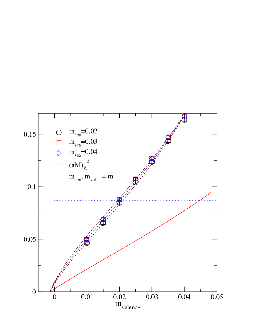
Figure 19: The pseudo-scalar meson mass, squared, extracted from the wall-point axial-vector correlation function. $m_{sea}=0.02$ (circles), 0.03 (squares), and 0.04 (diamonds). Dashed lines denote a next-to-leading order in chiral perturbation theory fit. The dotted line marks the mass of the kaon. The solid line shows the results of an extrapolation of the dynamical, and one of the valence, quark masses to $\bar{m}$. In this case the x-axis represents the remaining valence quark mass.

We begin by fitting the pseudo-scalar meson mass to Eqs. 34 and 36. To be fully consistent we should perform a simultaneous fit of $M_{PS}$ and $f_{PS}$ as both fit functions depend on $B_{0}$ and $f$. However, as we explain in the following, the $f_{PS}$ fit is problematic. As such, for the the $M_{PS}$ fit we use a fixed value of $af=0.078$, which is the result of a linear fit to the decay constant mass dependence. The results are summarized in Table 19 and, for the wall-point axial vector, shown in Figure 19. We have taken $\Lambda_{\chi}=1$ GeV; a change in this scale is absorbed into the scale-dependent $L_{i}$, leaving the value of $B_{0}$ unchanged. The NLO formula works well for quark masses up to about 0.04, where the fit quality begins to degrade. From Table 18, we note that a simple linear fit (lowest order in chiral perturbation theory) to the $m=m_{\rm sea}=m_{\rm val}$ points,

$$M_{PS}^{2}=c+b(m+m_{\rm res})\,,$$ (42)

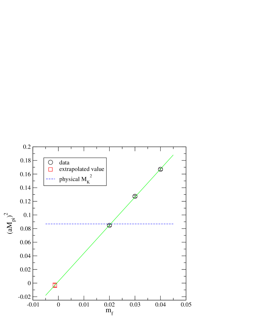
Figure 20: The pseudo-scalar meson mass squared, extracted from the wall-point axial-vector correlation function for the dynamical points ($m_{f}=m_{\rm sea}=m_{\rm val}$), together with the results of a LO chiral perturbation theory fit to the quark mass dependence. The experimental value for the square of the kaon mass is shown as a dashed line.

is consistent with the NLO fit. This fit and data are shown in Figure 20. In fact, the deviations from this simple linear form are quite small. However, so is the contribution of the logarithm predicted by NLO chiral perturbation theory. We conclude that our data are consistent with NLO chiral perturbation theory for $m_{f}\mathrel{\hbox to0.0pt{\raise 2.20013pt\hbox{$<$}\hss}{\lower 2.20013pt\hbox{$\sim$}}}0.04$.

The NLO fit is constrained to vanish in the chiral limit, $m_{f}=-m_{\rm res}$, as it must due to the universality of the low energy domain wall fermion theory Blum et al. (2004). Remarkably, the simple linear fit, which is not constrained, extrapolates to $m_{PS}^{2}\approx 0$ (within 1 standard deviation of the statistical error) at $m_{f}=-m_{\rm res}$ (see Figure 20). This is in stark contrast to the situation in the quenched approximation Blum et al. (2004); Aoki et al. (2004a), where the vanishing point from a simple linear extrapolation occurred when $m_{f}\approx-(2-3)\times m_{\rm res}$. This we attributed to the presence of quenched chiral logarithms, $\sim m_{PS}^{2}\,\ln{m_{PS}^{2}}$. Here Eq. 36 shows the chiral logarithms are much weaker, $\sim m_{PS}^{4}\,\ln{m_{PS}^{2}}$. Thus this comparison of the quenched and $N_{f}=2$ theories nicely confirms the predictions of chiral perturbation theory and the low-energy effective theory of domain wall fermionsBlum et al. (2004, 2002).

Another interesting feature of Figure 19 is that our simulations happen to coincide with the region where sea quark mass effects on $m_{PS}^{2}$ appear to be the greatest (in an absolute sense). Near the chiral limit, $m_{\rm sea}=$ constant curves approach each other since they must vanish at the same place, and as $m_{\rm val}$ gets heavy, they also merge since the heavy quarks are insensitive to the light sea quarks.

Now we discuss the determination of $\bar{m}$. $\bar{m}$ is found from the intersection of the NLO fit to $(am_{PS})^{2}$ with the line $(am_{PS})^{2}=(am_{\pi})^{2}$ where $m_{\pi}$ is the mass of the neutral pion, 134.9766 MeV, and the lattice spacing $a$ is set from the vector meson mass evaluated at $\bar{m}$. This procedure is performed iteratively until convergence (in practice the number of iterations $\mathrel{\hbox to0.0pt{\raise 2.20013pt\hbox{$<$}\hss}{\lower 2.20013pt\hbox{$\sim$}}}5$). We find $\bar{m}=0.00017(11)$. Similarly, we find $m_{DK}=0.0225(15)$ , where $m_{DK}$ is the quark mass for which a pseudo-scalar meson made of degenerate quarks has the same mass as the neutral kaon, $m_{K^{0}}=497.672$ MeV. Since the NLO formulas for $M_{K}^{2}$ and $f_{K}$ for non-degenerate valence quarks depend on the same parameters as in Eqs. 36 and 37, we make a determination of $m_{s}$ (and $f_{K}$) by extrapolating to this non-degenerate limitGolterman and Leung (1998a); Laiho and Soni (2002). These equations read:

$$\frac{\Delta M^{2}_{K}}{M^{2}_{K}} = \frac{-1}{N(M^{2}_{K}-M^{2}_{\pi})}\left[(M^{2}_{\pi}-M^{2}_{SS})A_{0}(M^{2}_{\pi})+(-2M^{2}_{K}+M^{2}_{\pi}+M^{2}_{SS})A_{0}(M^{2}_{33})\right]$$ (43)

$$-\frac{16}{f^{2}}[(L_{5}-2L_{8})M^{2}_{K}+(L_{4}-2L_{6})NM^{2}_{SS}]$$

$$\frac{\Delta f_{K}}{f} = \frac{1}{N16\pi^{2}f^{2}}(m^{2}_{K}-m^{2}_{SS})-\frac{m^{4}_{\pi}+m^{2}_{K}(m^{2}_{SS}-2m^{2}_{\pi})}{2N(m^{2}_{K}-m^{2}_{\pi})}\left(\frac{1}{m^{2}_{\pi}}A_{0}(m^{2}_{\pi})-\frac{1}{m^{2}_{33}}A_{0}(m^{2}_{33})\right)$$ (44)

$$-\frac{N}{2}(A_{0}(m^{2}_{uS})+A_{0}(m^{2}_{sS}))+\frac{8}{f^{2}}(L_{5}m^{2}_{K}+L_{4}Nm^{2}_{SS}),$$

$$M_{\pi}^{2} = 2B_{0}(\bar{m}+m_{\rm res})$$ (45)

$$M_{K}^{2} = B_{0}(\bar{m}+m_{s}+2m_{\rm res})$$ (46)

$$M_{33}^{2} = 2M_{K}^{2}-M_{\pi}^{2},$$ (47)

Note: Equations 36 and 43 have different logarithmic terms. The mass of the non-degenerate meson with one valence and both dynamical quark masses fixed to $\bar{m}$, is also shown in Figure 19, plotted versus the mass of the remaining valence quark. Thus, using Eq. 43 and the parameters determined from the degenerate formula, we find $m_{s}=0.0446(29)$, our final value. As a consistency check, we may take this value, together with the value for $\bar{m}$, and use the results of the partially quenched fit to the vector meson mass (Table 9) to estimate the mass of the $\phi$ meson. This gives a value of $M_{\phi}=978(12){\rm MeV}$; comfortably close to the experimental value of 1019 MeV. For comparison we have also extracted the strange quark mass from the linear fit. Using the three $m_{\rm sea}=m_{\rm val}$ points, one finds a value for the strange quark mass of $m_{s}=0.04177(64)$, $7\%$ smaller than the NLO value. The difference is easily appreciated from inspection of Figures 19 and 20 and demonstrates the significance of the NLO analysis in this case. Finally, it is important to note that $\bar{m}$ and $m_{s}$ as quoted above are bare quark masses that correspond to the physical $\pi$- and $K$- meson states; the renormalized quark mass is defined as $Z_{m}(m+m_{res})$, where $Z_{m}$ is a scheme and scale dependent renormalization factor.

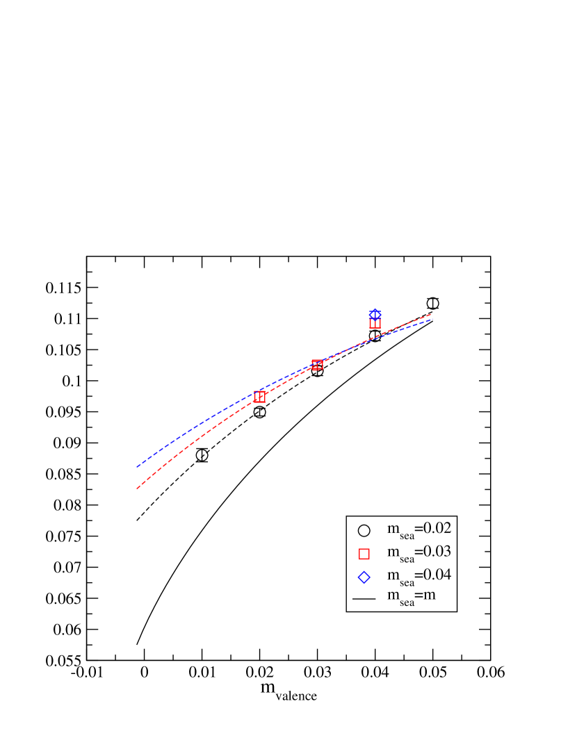
Figure 21: The meson decay constant. $m_{sea}=0.02$ (circles), 0.03 (squares), and 0.04 (diamonds). Dashed lines denote a next-to-leading order in chiral perturbation theory fit, with the solid line being the extrapolation to $m_{sea}=\overline{m}$.

We now move to the extraction of the decay constants from the point-point correlators. Recall that the errors on the decay constant from the axial-vector case are significantly larger than in the pseudo-scalar case, so we focus on the latter; our conclusions do not depend on this choice. In contrast to the above analysis for $m_{PS}^{2}$, the NLO chiral perturbation theory formula for the decay constant, Eqs. 36 and 37, does not fit the data. The results of this fit are presented in Table 20. Restricting $m_{f}\leq 0.03$, the resulting fit is shown in Figure 21. While it reproduces the data used in the fit reasonably well, it misses the larger mass points badly. Including these points in the fit does not change the fit results significantly except to increase the value of $\chi^{2}$. Note that the $m_{\rm sea}=\bar{m}$ line bends down steeply as $m_{\rm val}\to 0$ which yields a value for $f_{\pi}=100(10)$ MeV, $\sim 30$% smaller than the physical value.

There is just enough data to attempt a restricted NNLO fit, in which we include all of the ${\cal O}(p^{6})$ analytic terms: $C_{1}m^{2}_{\rm sea}$, $C_{2}m^{2}_{\rm val}$, and $C_{12}m_{\rm sea}m_{\rm val}$. This fit is not a systematic application of chiral perturbation theory, as we do not include the (un-calculated) logarithmic terms which also appear at this order. However, performing this fit allows us to investigate the utility of moving to the next order, and estimate the size of the terms needed. The results of the NNLO fit are summarized in Table 21. While the value of $\chi^{2}$ is acceptable, the errors on the fitted parameters are extremely large, especially in the case of $C_{1}$.

The basic problem is that the coefficient of the log term, which has been calculated analytically in the continuum (Eq. 37), is inconsistent with our data, which appears to be mostly linear. The additional NNLO terms in the fit do act to reduce the effect of this log, but this approach is both badly constrained and non-systematic. One interpretation of our data is that the quark masses we are using are sufficiently heavy that the NNLO terms are important relative to the NLO terms. In this case, the only way to do better is to simulate at even lighter values of the quark mass where (presumably) chiral perturbation theory works well.

There are several other interpretations: both lattice artifacts (${\cal O}(a^{2})$ in this study) and finite volume effects modify the coefficient of the chiral log, possibly making it smaller. In the former case we expect this effect to be of the order of a few percent, while including finite size effects such as the ones in Bernard (2002) should not change the fits significantly since our smallest mass still corresponds to $m_{PS}L\mathrel{\hbox to0.0pt{\raise 2.20013pt\hbox{$>$}\hss}{\lower 2.20013pt\hbox{$\sim$}}}3$. Neither of these effects therefore seem large enough to explain the discrepancy. In Aubin et al. (2004b), it is also suggested that using a physical parameter, such as $f_{K}$, as the chiral coupling rather than $f$, leads to a better behaved chiral expansion. This approach will have the effect of significantly reducing the coefficient of the chiral logarithm when applied to our data. If we allow the coefficient of the continuum chiral log to be free parameter in the NLO equation, then we are able to make a good fit ($\chi^{2}$/dof = $0.48(38)$). However, we find that this coefficient is $0.2(4)$, instead of the value 1 predicted by the continuum theory, which is a large deviation.

A remaining alternative is to forsake most of the higher order terms and do a simple linear fit. Again, this is not systematic, as this leaves out the (known) NLO logarithmic term. We fit the data with three independent terms, $f$, and terms proportional to $m_{\rm sea}$ and $m_{\rm val}$ (in other words, we simply set the coefficient of the log term in the NLO formula to zero):

$$f_{PS}=af+c_{1}\frac{m_{1}+m_{2}+2m_{\rm res}}{2}+c_{2}(m_{\rm sea}+m_{\rm res})$$ (48)

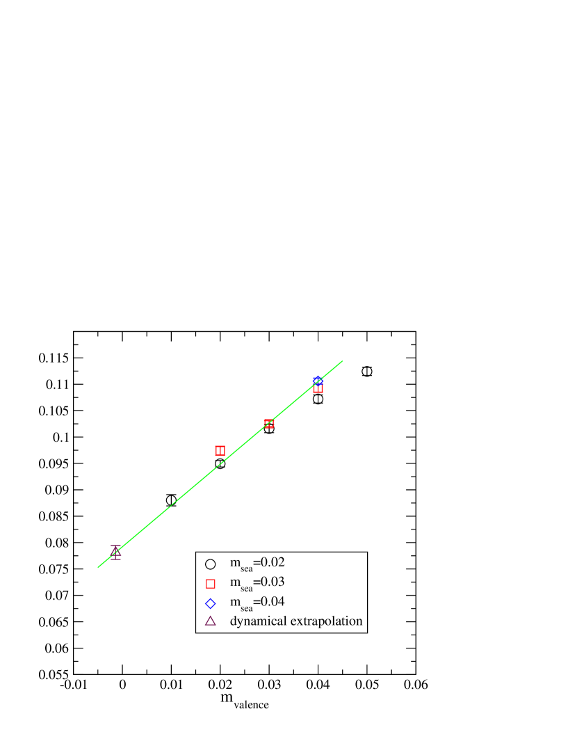
Figure 22: The meson decay constant. $m_{sea}=0.02$ (circles), 0.03 (squares), and 0.04 (diamonds), together with the results of a linear fit to the dynamical points. The extrapolated value at $m_{sea}=-m_{\rm res}$ is also shown.

As mentioned before, such a fit – the results of which we summarize in Table 22 and Figure 21 – actually describes the data quite well. For comparison, $f$ is also extracted from a simple two parameter linear fit to the $m_{sea}=m_{val}$ data points (see Table 22 and Figure 22); these two linear fits agree well. Using the three parameter linear fit, restricted to $m_{val}\leq 0.04$, we find $f_{\pi}=134.0(42)$ MeV, $f_{K}=157.4$(38) MeV, and $f_{K}/f_{\pi}=1.175(11)$, while the Particle Data Book gives $f_{\pi}=130.7$ MeV, $f_{K}=160$ MeV, and $f_{K}/f_{\pi}=1.224$.

While the inability to fit our data to the predicted NLO chiral perturbation theory form is discouraging, it is not unprecedented: this problem also exists for the current Wilson fermion Aoki et al. (2003); Ali Khan et al. (2002), and staggered fermion Aubin et al. (2004b) simulations. The former simulations, for dynamical masses in the range such that $M_{\pi}/M_{\rho}=0.6-0.8$, saw little evidence for the existence of the chiral log, extracting final numbers using a polynomial ansatz for the mass dependence (Hashimoto et al. (2003) discusses the matter further). The latter simulations, which include much lighter dynamical masses, also cannot fit the NLO formula for comparable quark masses. They quote final results from a restricted NNLO fit which, as above, leaves out the logarithmic terms that should appear at that order. The advantage of this work, however, is that we have a much cleaner extraction of the decay constants due to both flavour and chiral symmetry being respected at finite lattice spacing, allowing us to be confident that this discrepancy from continuum NLO chiral perturbation theory is a physical effect.

V.2 Static quark potential

In this section we discuss the extraction of the static quark potential, $V(r)$, from the Wilson loop, $W(\vec{r},t)$. To improve the signal we smear the operator in the spatial coordinates using $n_{smear}$ applications of APE smearingAlbanese et al. (1987),

$$U^{\prime}_{i}(x)\leftarrow{\rm Proj_{SU(3)}}\left[U_{i}(x)+c_{smear}U^{(staple)}_{i}(x)\right]\ \ \ (i=1,2,3)\ ,$$ (49)

where $U^{(staple)}_{i}(x)$ is the sum of four spatial staples. Using these smeared links we construct the spatial path between the infinitely heavy quark and anti-quark by employing the Bresenham algorithm Bolder et al. (2001).

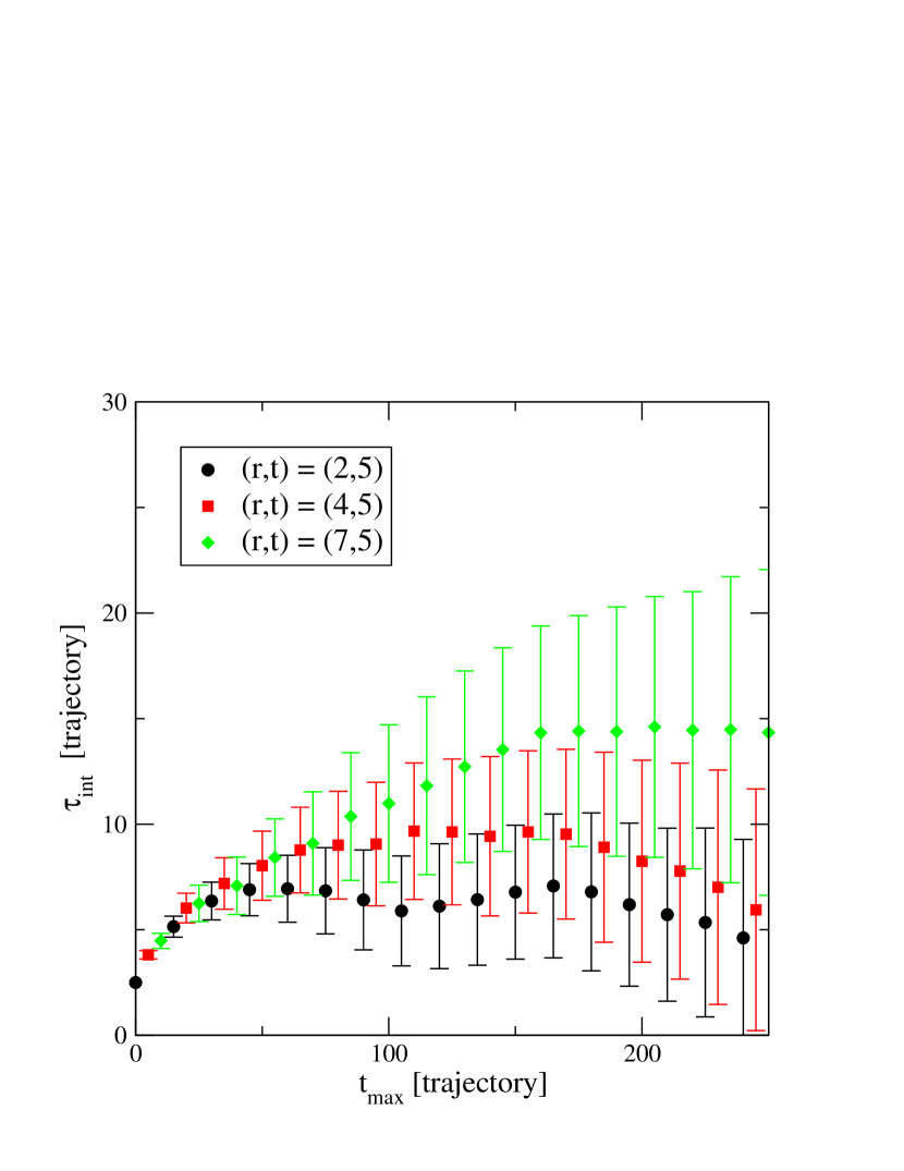
Figure 25: The integrated autocorrelation time, $\tau_{int}$, of the Wilson loops, $\left\langle W(r,t)\right\rangle$, for $m_{sea}=0.02$.

To cut down on short-term noise, we measure the static quark potential more frequently than every 50 trajectories, although our final results are obtained from a block-average over 50 trajectories. Fig. 25 shows the integrated autocorrelation times of a selection of Wilson loops, which are $\leq 25$ trajectories for $r\leq 8$. In total we use 941, 559 and 473 configurations for $m_{\rm sea}=0.02,0.03$ and $0.04$ respectively; these configurations are separated by five trajectories for $m_{\rm sea}=0.02$, while one in every ten trajectories is measured for $m_{\rm sea}=0.03$ and 0.04. Trajectories from 1775th to 2025th of $m_{\rm sea}=0.04$ are abandoned due to the hardware error described in Section IV.

We use the theoretical formula

$$\frac{\left\langle W(\vec{r},t)\right\rangle}{\left\langle W(\vec{r},0)\right\rangle}=C(\vec{r})\exp[-V(\vec{r})t]$$ (50)

which should hold for large $t$, and (following Aoki et al. (2004a)) extract $V(\vec{r},t)$ from

$$V(\vec{r})=\log\left[\frac{\left\langle W(\vec{r},t)\right\rangle}{\left\langle W(\vec{r},t+1)\right\rangle}\right]~{}~{},$$ (51)

together with $C(\vec{r})$ from

$$C(\vec{r})={\frac{\left\langle W(\vec{r},t)\right\rangle^{t+1}}{\left\langle W(\vec{r},0)\right\rangle\left\langle W(\vec{r},t+1)\right\rangle^{t}}}\ .$$ (52)

To maximize the overlap factor, $C(\vec{r})$, we have explored the two dimensional parameter space for the smearing, $(c_{smear},n_{smear})$, in the range $0\leq c_{smear}\leq 1$, $0\leq n_{smear}\leq 60$. We conclude $(c_{smear},n_{smear})=(0.5,20)$ is a reasonable choice for all of $r$ we use.

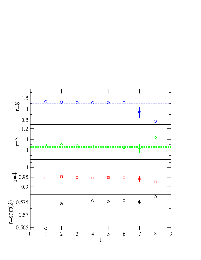
Figure 26: The static quark potential of $m_{sea}=0.02$ at $r$,extracted using Eq. 51 at $t$ shown as the horiozntal axis in the graph.$r=\sqrt{2},4,5,$ and 8.

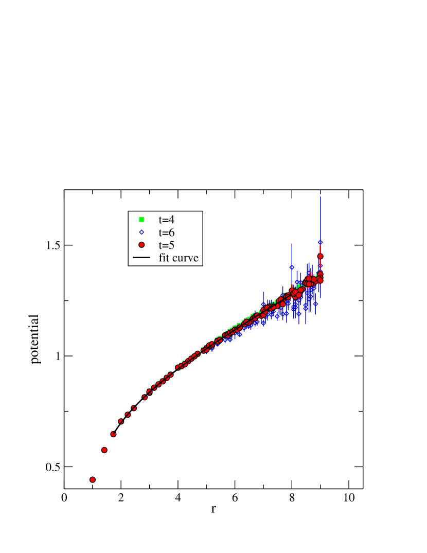
Figure 28: The static quark potential extracted from $t=4,5$ and 6 for $m_{sea}=0.02$. The black curve is the fit result to Eq. 55 with $l=0$ using $t=5$ and $\sqrt{3}\leq r\leq 8$.

The dependence of the potential to the temporal length of the Wilson loop is carefully examined to control the contamination from excited states. We found $V(\vec{r})$ and $C(\vec{r})$ extracted from $t\geq 5$ and $r\leq 8$ is relatively independent of $t$, and we therefore extract our results from this range. This can be clearly seen in Figure  26, which shows $V(\vec{r})$ for $m_{\rm sea}=0.02$. The effect of the positivity violation in improved gauge actionsLuscher and Weisz (1984) for small $t$ is evident in the graph: $V(r)$ extracted from $t<3$ approaches its asymptotic value from below for $r=\sqrt{2}$. This was also observed in quenched simulations Necco (2004), and the effect on $C(\vec{r})$ is discussed in Hashimoto and Izubuchi (2004); Iwasaki et al. (1997); our selection of temporal length is set as large as possible to exclude this lattice artifact. The potential extracted from $t=4,5$ and 6 is shown in Fig. 28 for the $m_{\rm sea}=0.02$ ensemble versus $r$. We see no evidence of string-breaking for large $r$.

For ease of comparison with other work, we also fit the potential to the form

$$V(\vec{r})=V_{cont}(r)-l\delta V(\vec{r}),~{}~{}r=|\vec{r}|\ ,$$ (53)

$$\ \ \ V_{cont}(r)=V_{0}-{\frac{\alpha}{r}}+\sigma r\ ,$$ (54)

$$\ \ \ \delta V(\vec{r})=\left[{\frac{1}{\vec{r}}}\right]-{\frac{1}{r}}\ ,$$ (55)

where $[{1/\vec{r}}]$ is the lattice Coulomb potential Michael (1992); Lang and Rebbi (1982); Weisz (1983); Iwasaki and Yoshie (1984),

$$\left[\frac{1}{\vec{r}}\right]=\int_{-\pi}^{\pi}\frac{dk^{3}}{8\pi^{2}}\frac{\exp(i\vec{k}\cdot\vec{r})}{\sum_{i}\sin^{2}(k_{i}/2)-4c_{1}\sum_{i}\sin^{4}(k_{i}/2)}\,.$$ (56)

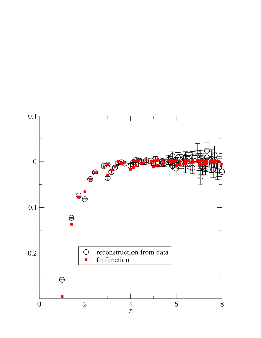
Figure 27: $\delta V_{L}(\vec{r})$ and its corresponding reconstruction from fit data, $[V^{\rm(data)}(\vec{r})-V_{cont}(r)]/l$. Data extracted on $m_{sea}=0.02$ configuration at $t=5,r\in[\sqrt{3},8]$ is used in the fit.

This form is often used in an attempt to correct the breaking of the rotational symmetry of the lattice. The correction term, $\delta V(\vec{r})$, describes the corresponding data, $[V^{\rm(data)}(\vec{r})-V_{cont}(r)]/l$, qualitatively well as seen in Figure 27, in which $V_{cont}(r)$ and $l$ are from the fit result using $t=5,r\in[\sqrt{3},8]$ on $m_{sea}=0.02$ ensemble. We also note that the fit parameters, especially $\alpha$, become less sensitive to the selection of $r_{min}$ by adding the lattice Coulomb term, although the errors become larger.

The fit results (both with and without the lattice Coulomb term), together with Sommer scaleSommer (1994),

$$r_{0}=\sqrt{\frac{1.65-\alpha}{\sigma}}\ ,$$ (57)

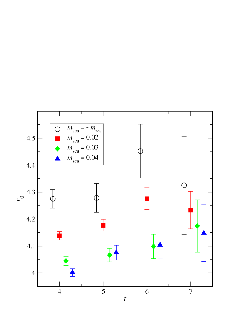
Figure 29: $t$ dependence of the Sommer scale $r_{0}$ for $m_{sea}=0.02,0.03,0.04$ as well as the lineary extrapolated value at chiral point, $m_{sea}=-m_{res}$. The fit formula with the lattice Colomb term correction ,Eq. 55 with $l\neq 0$, are used.

are presented in Table. 23. As can be seen in Figure 29, a major source of systematic error is the selection of $t$, with the $r_{max}$ dependence being almost negligible. To be precise, one can see a mild but continuous increase of $r_{0}$ as $t$ becomes large. At $t=7$, the signal to noise ratio becomes poor, and the statistical error of the data at $t=6$ is less controlled as seen in Figure 26. We therefore choose to take our central values from $t=5$ and $r\in[r_{min},r_{max}]=[\sqrt{3},8]$, quoting a systematic error due to the selection of $t$, as well as fit range by the shift of central values of these parameters. The selection is varied in either direction in $t,r_{min},r_{max}$ at once. The fit ranges $r_{min}\in[\sqrt{2},\sqrt{6}]$, $r_{max}\in[7,9]$, and $t=5,6$ are swept. More detailed results including the direct evaluation of the force, $\nabla V(\vec{r})$, and comparison with quenched simulation will be presented elsewhere Hashimoto and Izubuchi (2004); Hashimoto (2004).

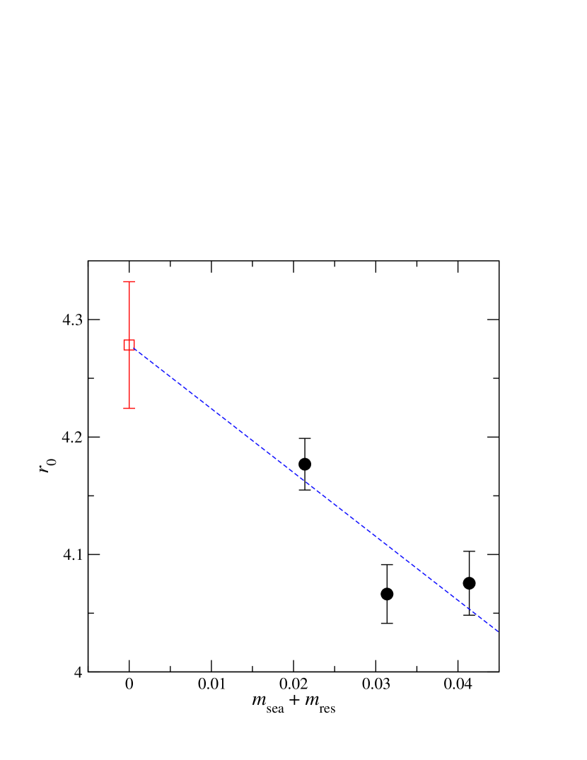
Figure 30: Sommer scale $r_{0}$ as a function of $m_{sea}$ and their chiral extrapolation using linear function. Error bars are statistical only.

Although in this paper we use the hadronic observables to set the lattice scale, we may also set the scale from $r_{0}$. The sea quark mass dependency of $r_{0}$ is shown in Figure 30. This mass dependence is consistent with that observed using other fermion formulations Allton et al. (1999a); Bali et al. (2000); Bernard et al. (2000); Ali Khan et al. (2002); Aoki et al. (2003). Linearly extrapolating to the chiral limit, we obtain a value of $r_{0}$ in lattice unit of

$$r_{0}|_{m_{sea}\to-m_{res}}=4.278(54)\left({}^{+174}_{-011}\right)~{}~{}.$$ (58)

This value is obtained from the fit without the lattice Coulomb term and the systematic error in the second parenthesis is estimated by the various choice of fit ranges. We note that the large positive shift of the central value (+174) is due to the rise of the $r_{0}$ at $r_{min}=\sqrt{3}$ from $t=5$ to $t=6$. This could be a sign of the remaining excited states contamination but it is less conclusive with the comparably large statistical error at $t=6$ as seen in Figure 29. We note that $r_{0}$ depends on $m_{\rm sea}$ so mildly that linear fit of $1/r_{0}$ yields a very close value, $r_{0}|_{m_{\rm sea}\to-m_{\rm res}}=4.287(58)$, at the chiral limit. The fit with the lattice Coulomb term yields similar value, $r_{0}=4.235(56)$. All of these three numbers are within the quoted statistical error.

For our final results we use the continuum fitting form, and a linear fit to the mass dependence; taking $r_{0}=0.5$ fm we get

$$a^{-1}_{r_{0}}=1.688(21)\left({}^{+69}_{-04}\right)\mbox{\rm GeV}~{}~{},$$ (59)

which, in contrast to the situation in the quenched approximationAoki et al. (2004a), is consistent with the value, $a_{\rho}^{-1}=1.691(53){\rm GeV}$, extracted from the rho meson mass.

V.3 Kaon B parameter

When studying the mixing of neutral kaon in the standard model, it is necessary to calculate the low energy matrix element, in QCD, of the effective weak interaction operator

$$O_{LL}=\bar{s}\gamma_{\mu}(1-\gamma_{5})d\,\bar{s}\gamma_{\mu}(1-\gamma_{5})d\,,$$ (60)

between kaon states. This is usually quantified in terms of the kaon B-parameter,

$$B_{K} = \frac{\langle\bar{K^{0}}|\bar{s}\gamma_{\mu}(1-\gamma_{5})d\,\bar{s}\gamma_{\mu}(1-\gamma_{5})d|K^{0}\rangle}{\frac{8}{3}\,\langle\bar{K^{0}}|A_{4}|0\rangle\langle 0|A_{4}|K^{0}\rangle},$$ (61)

$$= \frac{\langle\bar{K^{0}}|\bar{s}\gamma_{\mu}(1-\gamma_{5})d\,\bar{s}\gamma_{\mu}(1-\gamma_{5})d|K^{0}\rangle}{\frac{8}{3}\,f_{K}^{2}\,M_{K}^{2}}.$$ (62)

Before describing the lattice calculation of $B_{K}$, we address the (unphysical) mixing of $O_{LL}$ with wrong chirality dimension six operators. Such mixings are allowed in the chiral limit due to the explicit breaking of chiral symmetry of domain wall fermions with finite $L_{s}$. However, since such explicit breaking is small, it is useful to understand the order of magnitude of these mixings in terms of $am_{\rm res}$. This allows us to argue they may be neglected in our calculation. The framework for understanding this mixing within a low energy effective theory of domain wall fermions was laid out in Blum et al. (2004, 2002), but there the explicit example of $B_{K}$ was not discussed. We begin by adding a spurion field $\Omega$ to the low energy effective action for domain wall fermion QCD, whose only effect is to modify the symmetry breaking terms in the action so they transform in the same way as a conventional mass term. Each spurion field in the modified action or effective weak operator carries a factor of $am_{\rm res}$. After determining the dependence of the correlation function on $\Omega$, and therefore $am_{\rm res}$, we set $\Omega\to 1$ to recover the low energy theory of domain wall fermions. In the exact theory, the original four-quark operator transforms as a (27,1) dimensional representation of $SU_{L}(3)\times SU_{R}(3)$ chiral symmetry which must also be true for the modified wrong chirality operators if they are to mix. All such operatorsAllton et al. (1999b) have at least two right-handed quark fields, so at least two spurion fields are needed to formally rotate these into left-handed fields. Thus, to lowest order the mixing is $\sim(am_{\rm res})^{2}$, or ${\cal O}(10^{-6})$; this is small enough that it may be neglected in the present calculation. We note that the leading explicit chiral symmetry breaking in the matrix element is still ${\cal O}(am_{\rm res})$, however. This is just the statement that the chiral limit for all low energy observables is $m_{f}=-m_{\rm res}$Blum et al. (2004). Once this trivial shift is taken into account, the error on $B_{K}$ is again ${\cal O}((am_{\rm res})^{2})$.

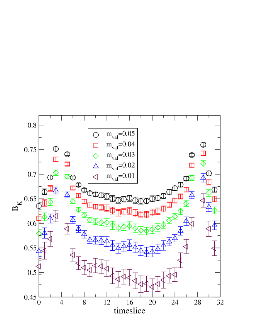
Figure 31: The pseudo-scalar B parameter for $m_{sea}=0.02$ and a range of degenerate valence quark masses versus the time-slice of the operator insertion.

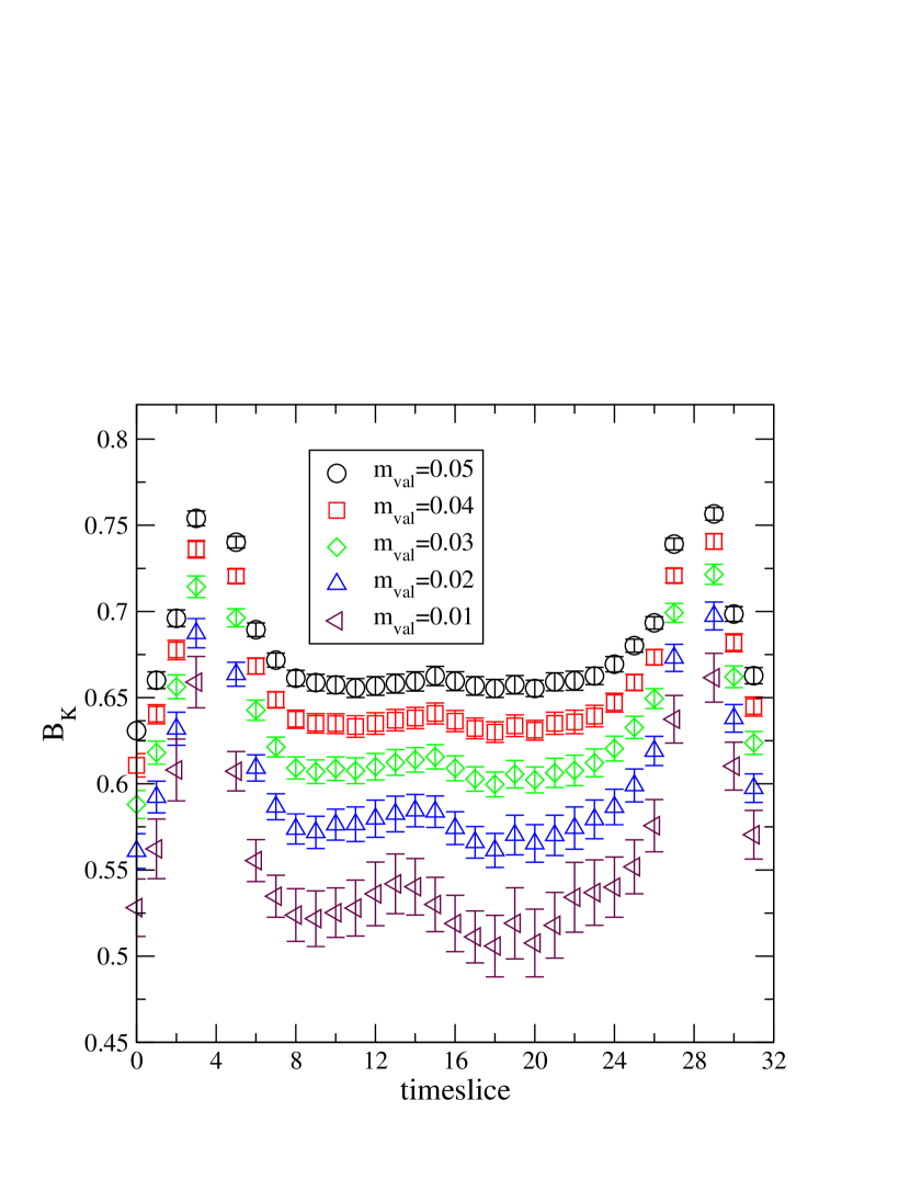
Figure 32: The pseudo-scalar B parameter for $m_{sea}=0.03$ and a range of degenerate valence quark masses versus the time-slice of the operator insertion.

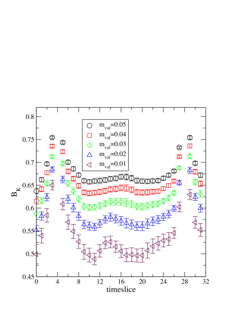
Figure 33: The pseudo-scalar B parameter for $m_{sea}=0.04$ and a range of degenerate valence quark masses versus the time-slice of the operator insertion.

Details of the method used to calculate $B_{K}$ can be found in Blum et al. (2003). We employ the so-called conventional method (Eq. 61), since difficulties of the quenched approximation, such as significant contamination by topological near-zero modes, do not apply Blum et al. (2003). The lattice B parameter for arbitrary quark mass, denoted $B_{PS}$, is tabulated in Tables 24 and 25-27, for degenerate and non-degenerate valence quark masses respectively. The values shown are averages over the time slice range for the operator insertion, $t_{op}=14-17$. The source and sink pseudo-scalar meson time slices were fixed to $t=4$ and 28, respectively. These values were chosen based on the quenched calculation in Blum et al. (2003) ($a^{-1}\approx 2$ GeV) where they lead to reasonable plateaus, which is also the case here (we also averaged the value of $B_{PS}$ over a larger time slice range, $t_{op}=10-22$, and found good agreement in all cases). This can be seen in Figures 31-33. Note however, that there are large fluctuations in the plateaus for the smallest valence quark masses.

To extract $B_{K}$, we fit our data for $B_{PS}$ to the predictions of NLO chiral perturbation theory, and extrapolate/interpolate to the physical quark masses. Our preferred way to do this is, of course, to take the (non-degenerate ) limit

$$m_{\rm sea}\rightarrow\overline{m}\ ;\ m_{\rm val,1}\rightarrow m_{s}\ ;\ m_{\rm val,2}\rightarrow\overline{m}\,,$$ (63)

corresponding to dynamical, degenerate up and down quarks, and a quenched strange quark. However, as previous work has only used degenerate valence quark masses, extrapolating to the point

$$m_{\rm val,1}\equiv m_{\rm val,2}=m_{DK}\,,$$ (64)

we also present results from this method, so we may compare the two techniques.

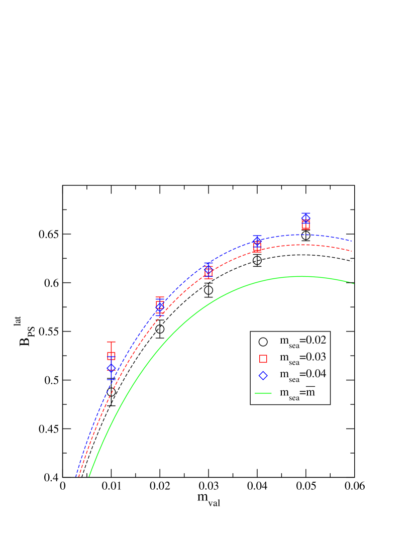
Figure 34: The pseudo-scalar B parameter, extracted from time-slices 14 to 17; $m_{\rm sea}\neq m_{\rm val}$. $m_{\rm sea}=0.02$ (circles), 0.03 (squares), and 0.04 (diamonds). The dashed lines are from a fit to Eq. 65, evaluated at $m_{\rm sea}=0.04$, 0.03, 0.02, and the solid line is an extrapolation, in the dynamical mass, to $\bar{m}$. The range of quark masses used in this particular fit is $0.02\leq m_{f}\leq 0.04$.

The degenerate valence quark mass data is plotted in Figure 34. As can be seen, $B_{PS}$ displays a rather weak, but noticeable, dependence on the sea quark mass. To be precise: as $m_{sea}$ decreases so does $B_{PS}$. The predicted dependence of $B_{PS}$ on $m_{sea}$ and $m_{val}$, when $m_{sea}\neq m_{val}$, is

$$B_{PS} = b_{0}\left(1-\frac{1}{(4\pi f)^{2}}\left(6\,M^{2}\,\log{\frac{M^{2}}{\Lambda_{\chi}^{2}}}\right)\right)+(b_{1}-b_{3})M^{2}+b_{2}M^{2}_{SS}\,.$$ (65)

Fits using Eq. 65 are summarized in Table 28. Eq. 65 does not simultaneously fit all of the data very well. This is evident from Figure 34: the results of the fit for $0.02\leq m_{\rm val}\leq 0.04$ are shown, and under-predicts both the lightest and heaviest points. However, as noted previously, we see large fluctuations in the plateau for the lightest valence quark masses, and the systematic error on these points probably outweighs the quoted statistical error. Therefore, for our final results we exclude both the $m_{\rm val}=0.01$ and $m_{\rm val}=0.05$ points; the latter in an attempt to stay in the region for which NLO chiral perturbation theory is valid.

We now move to the extraction of $B_{K}$ including the effect of non-degenerate valence quarks. In this case sea quark dependent log terms appear, as well as many new non-degenerate valence quark terms:

$$B_{PS} = b_{0}\left(1+\frac{M^{2}_{12}}{(4\pi f)^{2}}\left(-2(3+\epsilon^{2})\log{\frac{M^{2}_{12}}{\Lambda_{\chi}^{2}}}-(2+\epsilon^{2})\log{(1-\epsilon^{2})}-3\epsilon\log{\frac{1+\epsilon}{1-\epsilon}}\right)\right.$$

$$\left.+\frac{2}{3}\frac{1}{(4\pi f)^{2}}\left(\frac{3}{N}M_{SS}^{2}\left(\frac{2-\epsilon^{2}}{2\epsilon}\log{\frac{1+\epsilon}{1-\epsilon}}-2\right.\right.\right)$$

$$\left.\left.+\frac{3}{N}\,M^{2}_{12}\left(2+\epsilon^{2}-\frac{1-2\epsilon^{2}-\epsilon^{3}}{\epsilon}\log{\frac{1+\epsilon}{1-\epsilon}}+2\epsilon^{2}\log{\frac{M^{2}_{12}(1-\epsilon)}{\Lambda_{\chi}^{2}}}\right)\right)\right)$$

$$+b_{1}\,M_{12}^{2}+b_{2}\,M_{SS}^{2}+b_{3}\,M_{PS}^{2}(-2+\frac{M_{PS}^{2}}{M^{2}_{12}})\,.$$

In the above

$$\epsilon \equiv \frac{m_{2}-m_{1}}{m_{1}+m_{2}+2m_{\rm res}},$$ (67)

$$M_{PS}^{2} \equiv 2B_{0}\,(m_{1}+m_{\rm res}),$$ (68)

$$M_{12}^{2} \equiv 2B_{0}\frac{m_{1}+m_{2}+2m_{\rm res}}{2},$$ (69)

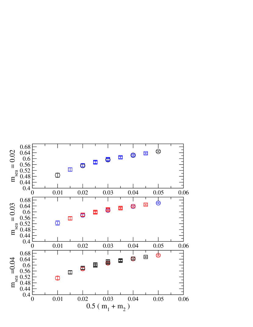
Figure 35: The pseudo-scalar B parameter; including non-degenerate valence quarks, $m_{1}\neq m_{2}$ (squares), and degenerate valence quark masses (circles).

where $m_{1}$, $m_{2}$ ($m_{1}\leq m_{2}$) are the valence quark masses. The log terms were computed in Golterman and Leung (1998b). $B_{PS}$ is shown in Figure 35 for both the degenerate and non-degenerate mass points, plotted as a function of $(m_{1}+m_{2})/2$. As can be seen, the non-degenerate points appear to lie on a smooth line connecting the degenerate mass points, a clear sign that the non-degenerate mass effects are small. Fits to Eq. V.3 are summarized in Table 29. Note that the value of $B_{K}$ is determined from the fit to Eq. V.3 evaluated at $m_{s}$ and $\bar{m}$. As in the degenerate case, we use valence quark masses in the range $0.02\leq m_{\rm val}\leq 0.04$ for the extraction of our final result.

It is customary to quote $B_{K}$ in the NDR-$\overline{MS}$ scheme at $\mu=2$ GeV. We accomplish this in two steps. First we renormalize non-perturbatively in the RI scheme at a scale $\mu\sim 1/a$ Izubuchi (2004) (Note that this extraction makes use of the pertubative two-loop, continuum, results for the running ), and then match to $\overline{MS}$ in the continuum using one-loop perturbation theory Ciuchini et al. (1995). Details of our method are given in Aoki et al. (2004c); Izubuchi (2004). With $Z^{\overline{MS}}_{B_{K}}=0.93(2)$ Izubuchi (2004) we find (adding errors in quadrature)

$$B_{K}^{\overline{MS}}(2\,{\rm GeV}) = 0.509\,(18).$$ (70)

for the degenerate case, and

$$B_{K}^{\overline{MS}}(2\,{\rm GeV}) = 0.495\,(18),$$ (71)

for the non-degenerate case. We take this as our final value for $B_{K}$. While these two numbers agree within the quoted statistical error, taking the jackknife difference shows that the 3% difference between the non-degenerate and degenerate extraction is statistically well resolved.

This two flavor, non-degenerate valence quark result is roughly 10% smaller than recent quenched values obtained with domain wall or overlap fermions Ali Khan et al. (2001b); Blum et al. (2003); DeGrand (2004); Aoki et al. (2004c) and roughly 20% smaller than the quenched values reported in Aoki et al. (1998); Garron et al. (2004) (Kogut-Susskind and overlap fermions, respectively). We caution that there are as yet unquantified systematic errors in our determination of $B_{K}$, most notably non-zero lattice spacing and finite volume effects. Recent quenched studies Ali Khan et al. (2001b); Aoki et al. (2004c) find these to be on the order of 5% each, though they could differ in the dynamical case.

Of course, the quantity of direct relevance to experiment is $B_{K}$ at the kaon mass, as quoted. However, in passing, we also mention our value for this parameter in the chiral limit, $B_{K}^{\chi}(\overline{MS},{\rm 2GeV})$, as it provides a useful comparison with phenomenological models Bijnens and Prades (1995); Peris and de Rafael (2000); Cata and Peris (2003), where calculations in the chiral limit are often under better control. We find, $B_{K}^{\chi}(\overline{MS},{\rm 2GeV})=0.241(10)$. This should be compared with a value of 0.267(14), obtained in our previous quenched study Blum et al. (2003).

In summary: our study shows that the inclusion of sea quarks and non-degenerate valence quarks tends to lower the value of $B_{K}$ by roughly 10% and 3%, respectively, which represents a very important step in estimating systematic uncertainties in $B_{K}$. We note that some time ago $N_{f}=2$ staggered fermion calculations found no sea quark effects on $B_{K}$ outside of quoted errorsKilcup (1993); Ishizuka et al. (1993). These studies used unimproved staggered fermions which have large lattice spacing errors; thus we consider our new determination to be more reliable. It should also be noted that early Wilson fermion results Soni (1996), as well as the more recent Flynn et al. (2004) suggest a small decrease in $B_{K}$ when including the effects of dynamical quarks. In Sharpe (1997) the effect of sea quarks on $B_{K}$ was estimated in chiral perturbation theory from the difference of the chiral logs between the quenched and dynamical theories. This comparison suggested that the sea quark effects increase the value of $B_{K}$, however it assumed that the analytic terms remain the same between the quenched and dynamical theories and so, again, we consider our determination to be more reliable.

VI Chiral Symmetry

In this section we will discuss our understanding of the (relatively large) breaking of chiral symmetry observed in this work, starting with our choice of gauge action. As mentioned previously, the DBW2 gauge action has been used successfully in the quenched approximation to improve the chiral properties of domain wall fermions. To give an example: when comparing the Wilson, Iwasaki, and DBW2 actions for inverse lattice spacings of approximately 2GeV, the residual masses for $L_{s}=16$ are around 3MeV, 0.3MeV and 0.03MeV respectively Aoki et al. (2004a). This dramatic improvement can be ascribed to the interplay of the positively weighted plaquette term and the negatively weighted rectangle term leading to a strong suppression of dislocations of the lattice. While we would like to exploit this mechanism in the dynamical case, it is not a priori obvious what form of bare gauge action we should take such that, when combined with the effects of the fermion determinant, we have an effective short-distance gauge action with a similar form to that used in the quenched approximation. Over large (physical) distance scales it is well-known that the effect of adding the determinant is to smooth out the gauge field, and so, in order to perform a dynamical simulation with the same lattice spacing as a quenched simulation, we must increase the gauge coupling. The question we are interested in here, however, is how the inclusion of the fermion determinant modifies the short-distance properties of the gauge field. One particular worry, for example, is that the addition of the fermion determinant may effectively induce a rectangle term of the opposite sign to the one in the gauge action, leading to reduced suppression of dislocations.

To study this we solve for the short distance effective gauge action using the Schwinger-Dyson equations, following the approach of de Forcrand et al. (2000). Briefly summarizing: for an ansatz of the effective gauge action of

$$S=\beta^{\alpha}S^{\alpha}\,,$$ (72)

a set of operators, $O_{i}$, and some variation of the gauge fields, $\delta$, the Schwinger-Dyson equations read

$$\langle\delta O_{i}\rangle=-\langle O_{i}\left[\delta S^{\alpha}\right]\rangle\beta^{\alpha}\,.$$ (73)

Calculating $\langle\delta O_{i}\rangle$ and $\langle O_{i}\left[\delta S^{\alpha}\right]\rangle$ for the same number of independent operators as there are independent terms in the ansatz for the gauge action, this equation may be solved to give $\beta^{\alpha}$. In the following we use

$$S^{\alpha}=1-\frac{1}{3}\sum_{l}{\rm Re}{\rm Tr}\left[U_{l}G_{l}^{\alpha}\right]$$ (74)

where $U_{l}$ denotes a specific link and $G_{l}^{\alpha}$ the sum of the (forward) staples of type $\alpha$ for link $l$, and the variation

$$\delta^{a}_{l}U_{l}=-i\epsilon^{a}\lambda^{a}U_{l}$$ (75)

for observables

$$O^{a,i}_{l}={\rm Im}{\rm Tr}\left[\lambda^{a}U_{l}G_{l}^{i}\right]\,,$$ (76)

and then sum Eq. 73 over $a$ and $l$.

Some idea of the utility of this method can be gained by studying quenched configurations. Obviously, should the ansatz of the gauge action include the terms that constitute the action used to generate the ensemble, then this is precisely the result this method will give. However, in Table 30 we show the results of applying this method using a quenched ensemble of 404 configurations of size $16^{3}\times 32$ generated with the DBW2 action with $\beta=1.04$ – corresponding to an inverse lattice spacing of $\approx 2{\rm GeV}$ – and solving for the effective plaquette gauge action. Using an observable based on the simple plaquette staple we get an answer of $\beta_{P}\approx 9$. An ensemble generated with this plaquette gauge action would have a much finer lattice spacing than the one we are studying; our interpretation of this result is that, at the short distances probed by this observable, lattices generated with the DBW2 action are much smoother than those of the same lattice spacing generated with the plaquette action. As can also be seen, as the size of the observable used to calculate the effective $\beta_{P}$ is increased to the $2\times 1$ planar rectangle; $2\times 2$ square and then $3\times 3$ square, the calculated value of $\beta_{P}$ decreases towards, presumably, the value that would generate one ensemble with the same lattice spacing as the one we are studying ($\beta\approx 6$).

Table 31 shows the results of applying this method to each of our dynamical ensembles, using relatively localized observables. In each case we see that the short distance properties of the gauge field are dominated by the bare form of the gauge action: the effective gauge action, up to some very small deviations, is identical to this bare gauge action. We may therefore qualitatively understand the larger observed chiral symmetry breaking for the dynamical lattices versus quenched lattices as being due to the smaller value of the (bare) $\beta$ used in the gauge action leading to reduced suppression of dislocations; the effects of the determinant seem to only become significant for larger distance observables.

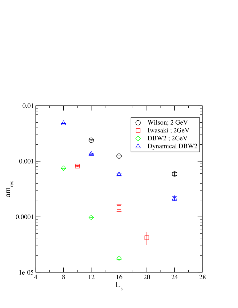
Figure 36: The residual mass versus $L_{s}$ for $m_{sea}=0.04$, compared with that measured on three quenched ensembles: Wilson $\beta=6.0$, Iwasaki $\beta=2.6$ and DBW2 $\beta=1.04$ ; all of which correspond to $a^{-1}\approx 2{\rm GeV}$.

While the chiral symmetry breaking observed for the ensemble studied here is small enough to be a negligible correction to the physical quantities we are calculating, it is still interesting to know how the residual mass varies both with the size of the fifth dimension and the gauge coupling. A reasonable estimate of the former may be made by calculating the residual mass for different valence values of $L_{s}$. Table 33 shows this for fifth dimension of extent 8 to 32 for the $m_{\rm sea}=0.04$ ensemble at the dynamical point. For $L_{s}\neq 12$ the residual mass is calculated on 45 configurations, leaving 100 trajectories between configurations starting from trajectory 1005 (we skip trajectories 1805 and 1905 due to the hardware error mentioned in Section IV). Figure 36 shows these dynamical results, and compares them with the residual mass on three quenched ensembles: Wilson $\beta=6.0$ Blum et al. (2004), Iwasaki $\beta=2.6$ Ali Khan et al. (2001a) and DBW2 $\beta=1.04$ Aoki et al. (2004a); all of which have inverse lattice spacings $\approx 2{\rm GeV}$. As can be seen, while the residual mass in the dynamical simulation is much larger than that in the comparable quenched DBW2 calculation, it is still smaller than the value when using the Wilson gauge action in the quenched approximation.

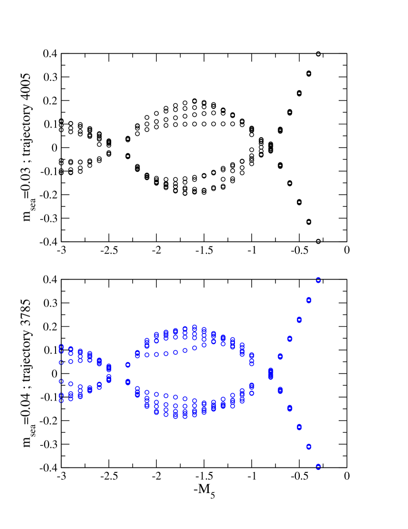
Figure 37: Two typical spectral flows: one from the $m_{sea}=0.03$ evolution and one from the $m_{sea}=0.04$ evolution.

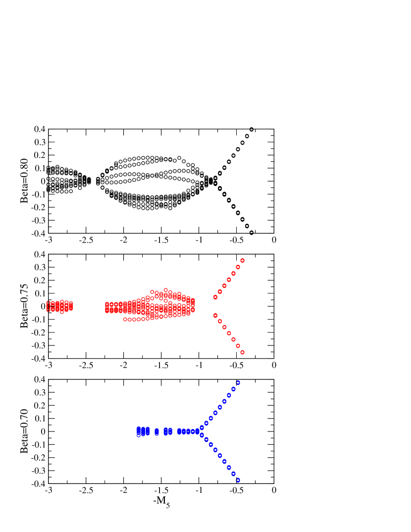
Figure 38: A comparison of three spectral flows: all generated with the DBW2 action, using $\beta=0.8$, $\beta=0.75$ and $\beta=0.7$ respectively.

We have also made a few exploratory studies using stronger couplings for the DBW2 gauge action in dynamical simulations Levkova and Mawhinney (2004), namely $\beta=0.75$ and $0.70$. For both these simulations we used $M_{5}=1.8$, $L_{s}=12$ on $16^{3}\times 32$ lattices, as with the rest of this work. Table 32 gives values of the input quark mass, number of configurations collected, the rho meson mass, and the value of the residual mass. As for each value of the coupling we used only one value for the dynamical quark mass, the latter two quantities are quoted in the valence chiral limit. While the residual mass at $\beta=0.70$ is not prohibitively large, caution should be taken; we may also look at at the spectral flow of the Hermitian Wilson Dirac operator. A transfer matrix in the fifth dimension for domain wall fermions may be written in terms of this operator, with the success of the domain wall fermion mechanism being dependent on the existence of a gap in the spectral flow for negative Wilson masses. Figure 37 shows a typical spectral flow for the $\beta=0.8$ ensembles, while Figure 38 shows typical spectral flows for all the gauge couplings we have studied. As can be seen, the gap in the spectral flow rapidly closes as we move to stronger gauge coupling. This is, perhaps, the main challenge for the domain wall fermion/overlap approach: the computational cost of lattice generation falls so quickly as the lattice spacing increases that the extra cost of domain wall fermions versus other approaches could easily be amortized by working on slightly coarser lattices. However, for the current formulation, the domain wall mechanism begins to fail as we move to lattice spacings significantly coarser then $a^{-1}\approx 2{\rm GeV}$. There have been some preliminary attempts to modify the gauge and/or fermion action in such a way that the domain wall mechanism persists at stronger couplings Levkova and Mawhinney (2004). These have so far met with limited success, but this is clearly a direction of research which has not been exhausted.

VII Conclusions

We have presented a large scale lattice QCD calculation using two flavors of dynamical domain wall fermions with small quark masses on lattices with large volumes. Domain wall fermions possess exact chiral symmetry in the limit $L_{s}\rightarrow\infty$ even at finite lattice spacing – a symmetry fundamental to much of the physics of QCD. The $\sim 3\times 5000$ Monte Carlo trajectories in this work obtained with light dynamical quarks and small residual quark mass, $m_{\rm strange}/2\mathrel{\hbox to0.0pt{\raise 2.20013pt\hbox{$<$}\hss}{\lower 2.20013pt\hbox{$\sim$}}}m_{\rm sea}+m_{\rm res}\mathrel{\hbox to0.0pt{\raise 2.20013pt\hbox{$<$}\hss}{\lower 2.20013pt\hbox{$\sim$}}}m_{\rm strange}$, represent a substantial computational undertaking that took almost two years to complete.

The first physics results to come from this endeavor are both interesting and encouraging. The decay constants $f_{\pi}=134.0(42)$ and $f_{K}=157.4(38)$ agree with experiment well within $\mathrel{\hbox to0.0pt{\raise 2.20013pt\hbox{$<$}\hss}{\lower 2.20013pt\hbox{$\sim$}}}$ 5% statistical errors. Their ratio, determined to 1% statistical accuracy, $f_{K}/f_{\pi}=1.175(11)$, slightly under-predicts the experimental value [1.223] obtained from the Particle Data Book.

The Kaon B parameter is the hadronic matrix element of the $\Delta S=2$ weak interaction operator that governs neutral kaon mixing. It is required to determine the level of indirect CP violation in the kaon system that is predicted in the Standard Model. We find that inclusion of sea quarks tends to decrease the value of $B_{K}$ relative to our comparable quenched calculationsBlum et al. (2003); Aoki et al. (2004c) by about two (statistical) standard deviations, or roughly 10%. Non-degenerate valence quark effects further lower the value by 3%. At a renormalization scale of 2 GeV in the continuum $\overline{MS}$ scheme, we find $B_{K}^{\overline{MS}}=0.495(18)$ (statistical error only) which is significantly lower than previously reported quenched values and could impact the extraction of the phase of Standard Model CKM quark mixing matrix if this value accurately describes the chiral, infinite volume and continuum limits.

Besides physical results, two important and closely related theories, the low-energy effective theory of domain wall fermions and (partially-) quenched chiral perturbation theory, are strongly supported by the pattern of explicit chiral symmetry breaking in our calculations. In quenched calculations the pion mass squared, when fit to a simple linear function of the quark mass, significantly over-shot the chiral limit, $m_{f}=-m_{\rm res}$. Through careful study, it was shown that this effect could be explained by a prediction of quenched chiral perturbation theory, that is to a logarithmic singularity unique to the chiral approximation. When accounting for this term, $m_{\pi}^{2}$ was shown to vanish at the correct chiral limit. In the two-flavor case this offending logarithm does not appear. Such a logarithm appears only at higher order (see Eq. 36) and does not effect the chiral limit. The net result is that a simple linear extrapolation of $m_{\pi}^{2}$ should come closer to the true chiral limit. That this indeed happens was demonstrated in Figure 19 and Table 19.

These initial results, obtained from two flavor calculations with three relatively heavy sea quark masses, on a single volume and lattice spacing, and fifth dimension $L_{s}=12$, while encouraging, may still suffer significant systematic uncertainties. We stress that the use of next-to-leading order partially-quenched chiral perturbation theory was crucial in our analysis of $m_{\pi}^{2}$ and $B_{K}$, where it worked reasonably well. The analysis for the decay constant was more problematic. This lead us to quote results for $f_{\pi}$ and $f_{K}$ from linear fits, i.e. the NLO analytic terms were included but not the logarithms. In addition, while the number of trajectories in our study is large from a historical perspective, large scale auto-correlations which can only be detected in longer runs may still be present. In fact, here as in all dynamical simulations, the number of trajectories studied is determined at least as much by the amount of available computer resources as by established scientic criteria. All of these issues must be further addressed by future calculations. The proven scaling behavior of domain wall fermions gives us confidence that the results presented here provide a solid foundation on which to build.

Tables

Table 1: Small lattice comparison of HMC evolutions. All these evolutions use the Wilson gauge action with $\beta=5.2$ and two flavours of Domain Wall Fermions with a bare mass of $m_{\rm sea}=0.02$.

Force Term	$\Delta t$	Steps/Trajectory	Trajectories	Acceptance	CG-iterations/Trajectory	$C_{\Delta H}$
Old	$1/64$	33	1000-1880	87%	8336	26.5
Old	$1/32$	17	1000-1929	59%	4310	30.0
New	$1/32$	17	1000-1936	79%	4179	12.9

Table 2: Parameters for the large lattice HMC evolutions. The averaged elapse time per one trajectory of our paricular implementation on 32 mother boards (32MB $\sim$ 100GFLOPS theoretical peak speed) or 64 mother boards (64MB $\sim$ 200GFLOPS) QCDSP, and the observed acceptance in the Metropolis test are also quoted. The CPU time includes the computation time for the chiral condensation, $\langle\bar{q}q\rangle^{L}_{m_{v}=m_{sea}}$, and the $r\times t$ on-axis Wilson loop, $\langle W(r,t)\rangle$ with $(r,t)=\{(1,1),(1,2),(2,1)\}$, but does not include the time for I/O. The scaled squared energy difference between the first and the last configuration in a trajectory, $C_{\Delta H}=\sqrt{\left\langle(\Delta H)^{2}\right\rangle/V}/(\Delta t)^{2}$, is quoted with the standard deviation error. “$0.02$ (OLD)” are the results of a small number of trajectories using the old force term.

$m_{\rm sea}$	$\Delta t$	Steps/Trajectory	Trajectories	Acceptance	$C_{\Delta H}$	Time/Trajectory(machine)
$0.02$ (OLD)	$1/100$	51	45	56%	39(4)
$0.02$	$1/100$	51	656-5361	77%	16.2(2)	0.8784(6) hours (64MB)
$0.03$	$1/100$	51	615-6195	78%	15.8(1)	0.8324(4) hours (32MB)
$0.04$	$1/80$	41	625-5605	68%	16.4(2)	0.7116(2) hours (32MB)

Table 3: Average cg-count and standard deviation (shown in square brackets) versus molecular dynamics step for trajectories 3000 to 4000 of each ensemble, together with the average for the total number of cg-iterations per trajectory.

Leapfrog step	$m_{\rm sea}=0.02$	$m_{\rm sea}=0.03$	$m_{\rm sea}=0.04$
$1/2$ step	715[11]	513.9[49]	401.5[32]
step 1	626[11]	435.0[49]	340.4[32]
step 2	543[11]	363.3[47]	284.7[29]
step 3	477[13]	297.6[50]	231.7[32]
step 4	411[19]	227.3[90]	172.3[48]
step 5	346[15]	181.1[61]	137.2[46]
step 6	280[12]	175.0[54]	128.2[41]
step 7	277[13]	157.9[58]	120.5[29]
step 8	269[10]	149.7[39]	117.8[21]
step 9	274[14]	146.0[60]	116.4[48]
step 10	275[15]	154.5[74]	115.6[51]
step 11	275[14]	158.3[47]	127.3[28]
step 12	269[17]	153.6[78]	122.0[65]
step 13	282[15]	152.6[76]	120.5[52]
step 14	279[17]	158.8[76]	122.1[51]
Total	16014[396]	9214[130]	5964[71]

Table 4: Evolution details and number of configuration used for physical results.

$m_{\rm sea}$	Until Accept/Reject	Thermalisation	Trajectories	Configurations
$0.02$	28	656	5361	94
$0.03$	25	615	6195	94
$0.04$	5	625	5605	94

Table 5: The bare chiral condensate, $\langle\bar{q}q\rangle^{L}_{m_{\rm val}=m_{\rm sea}}$, and the $r\times t$ on-axis Wilson loop, $\langle W(r,t)\rangle$.

$m_{sea}$	$N_{configs}$	$\langle\bar{q}q\rangle^{L}_{m_{val}=m_{sea}}$	$\langle W(1,1)\rangle$	$\langle W(2,1)\rangle$	$\langle W(2,2)\rangle$	$\langle W(3,3)\rangle$
0.02	94	0.002542(11)	0.646706(50)	0.407777(80)	0.17601(10)	0.033633(80)
0.03	94	0.0034419(98)	0.646594(47)	0.407629(82)	0.17572(10)	0.033287(81)
0.04	94	0.0043255(81)	0.646561(48)	0.407562(71)	0.175615(97)	0.033330(81)

Table 6: The fitted vector meson mass from the wall-point correlation function for $m_{\rm sea}=0.02$.

$m_{sea}$	$m_{val}$	fit range	$\chi^{2}/$dof	mass
0.02	0.01	5-16	$1.9(10)$	$0.511(10)$
0.02	0.015	5-16	$2.0(11)$	$0.5278(77)$
0.02	0.02	5-16	$1.8(11)$	$0.5425(64)$
0.02	0.025	5-16	$1.7(11)$	$0.5567(56)$
0.02	0.03	5-16	$1.6(11)$	$0.5712(50)$
0.02	0.035	5-16	$1.7(11)$	$0.5860(47)$
0.02	0.04	5-16	$1.9(11)$	$0.6010(44)$
0.02	0.045	5-16	$2.1(11)$	$0.6160(41)$
0.02	0.05	5-16	$2.3(12)$	$0.6309(39)$

Table 7: The fitted vector meson mass from the wall-point correlation function for $m_{\rm sea}=0.03$.

$m_{\rm sea}$	$m_{\rm val}$	fit range	$\chi^{2}/$dof	mass
0.03	0.01	6-16	$0.21(32)$	$0.537(13)$
0.03	0.015	6-16	$0.24(34)$	$0.5522(96)$
0.03	0.02	6-16	$0.37(42)$	$0.5669(79)$
0.03	0.025	6-16	$0.55(52)$	$0.5809(67)$
0.03	0.03	6-16	$0.75(62)$	$0.5946(58)$
0.03	0.035	6-16	$0.93(70)$	$0.6079(52)$
0.03	0.04	6-16	$1.07(76)$	$0.6213(47)$
0.03	0.045	6-16	$1.17(81)$	$0.6347(43)$
0.03	0.05	6-16	$1.25(85)$	$0.6481(40)$

Table 8: The fitted vector meson mass from the wall-point correlation function for $m_{\rm sea}=0.04$.

$m_{\rm sea}$	$m_{\rm val}$	fit range	$\chi^{2}/$dof	mass
0.04	0.01	7-16	$1.72(99)$	$0.580(25)$
0.04	0.015	7-16	$1.8(10)$	$0.586(19)$
0.04	0.02	7-16	$1.7(10)$	$0.591(15)$
0.04	0.025	7-16	$1.58(99)$	$0.598(11)$
0.04	0.03	7-16	$1.51(95)$	$0.6084(92)$
0.04	0.035	7-16	$1.47(95)$	$0.6198(79)$
0.04	0.04	7-16	$1.44(97)$	$0.6323(70)$
0.04	0.045	7-16	$1.41(99)$	$0.6455(64)$
0.04	0.05	7-16	$1.37(100)$	$0.6590(59)$

Table 9: The results of a fit to the quark mass dependence of vector meson mass.

fit	$\chi^{2}$/dof	$a$	$b$	$c$
dynamical	0.9 (19)	0.448(15)	4.52(47)
partially quenched	0.34(40)	0.448(13)	1.78(43)	2.78(13)

Table 10: The fitted nucleon mass from the wall-point correlation function.

$m_{\rm sea}$	$m_{\rm val}$	fit range	$\chi^{2}/$dof	mass
0.020	0.010	6-16	0.76 (69)	0.679 (19)
0.020	0.015	6-16	0.58 (62)	0.719 (12)
0.020	0.020	7-16	0.90 (80)	0.755 (12)
0.020	0.025	7-16	1.28 (96)	0.789 (10)
0.020	0.030	7-16	1.6 (1.1)	0.8209 (94)
0.020	0.035	7-16	1.8 (1.1)	0.8510 (89)
0.020	0.040	7-16	2.0 (1.1)	0.8796 (85)
0.020	0.045	7-16	2.1 (1.1)	0.9071 (83)
0.020	0.050	7-16	2.2 (1.1)	0.9338 (80)
0.030	0.010	7-16	1.43 (88)	0.747 (30)
0.030	0.015	7-16	1.29 (93)	0.766 (19)
0.030	0.020	7-16	1.13 (84)	0.788 (14)
0.030	0.025	8-16	1.14 (86)	0.816 (16)
0.030	0.030	8-16	1.05 (80)	0.844 (14)
0.030	0.035	8-16	1.01 (77)	0.870 (12)
0.030	0.040	8-16	1.02 (77)	0.896 (11)
0.030	0.045	8-16	1.06 (79)	0.922 (10)
0.030	0.050	8-16	1.12 (81)	0.9481 (95)
0.040	0.010	8-15	1.5 (1.1)	0.748 (44)
0.040	0.015	8-16	0.75 (70)	0.778 (35)
0.040	0.020	8-16	0.53 (56)	0.808 (25)
0.040	0.025	8-16	0.53 (59)	0.835 (19)
0.040	0.030	8-16	0.51 (60)	0.860 (15)
0.040	0.035	9-16	0.33 (54)	0.875 (15)
0.040	0.040	8-16	0.40 (52)	0.910 (11)
0.040	0.045	8-16	0.40 (53)	0.935 (10)
0.040	0.050	8-16	0.47 (59)	0.9602 (92)

Table 11: The $N^{*}$ mass from the wall-point correlation function.

$m_{\rm sea}$	$m_{\rm val}$	fit range	$\chi^{2}/$dof	mass
0.020	0.010	3-5	0.10 (67)	1.006 (46)
0.020	0.015	5-9	1.6 (1.4)	1.021 (92)
0.020	0.020	5-9	1.5 (1.4)	1.021 (71)
0.020	0.025	5-9	1.4 (1.3)	1.038 (59)
0.020	0.030	5-9	1.3 (1.3)	1.061 (50)
0.020	0.035	5-9	1.1 (1.2)	1.086 (42)
0.020	0.040	5-9	0.9 (1.1)	1.111 (37)
0.020	0.045	5-9	0.72 (99)	1.136 (32)
0.020	0.050	5-9	0.54 (87)	1.161 (28)
0.030	0.010	5-8	0.6 (1.2)	1.21 (75)
0.030	0.015	5-8	0.39 (90)	0.93 (12)
0.030	0.020	5-9	1.1 (1.3)	0.950 (65)
0.030	0.025	5-9	0.8 (1.1)	0.990 (48)
0.030	0.030	5-9	0.64 (98)	1.026 (38)
0.030	0.035	5-9	0.59 (93)	1.059 (32)
0.030	0.040	5-9	0.60 (93)	1.089 (28)
0.030	0.045	5-9	0.62 (94)	1.118 (25)
0.030	0.050	5-9	0.64 (95)	1.145 (23)
0.040	0.010	5-7	0.21 (97)	0.69 (17)
0.040	0.015	5-8	0.16 (63)	0.92 (10)
0.040	0.020	4-8	0.19 (52)	1.020 (47)
0.040	0.025	5-9	0.50 (84)	1.057 (49)
0.040	0.030	5-9	0.55 (88)	1.091 (39)
0.040	0.035	5-9	0.56 (88)	1.119 (33)
0.040	0.040	5-9	0.54 (87)	1.144 (28)
0.040	0.045	5-9	0.52 (85)	1.168 (25)
0.040	0.050	5-9	0.50 (84)	1.192 (23)

Table 12: Physical baryon mass at the light quark mass ($\bar{m}$) by diagonal ($m_{\rm val}=m_{\rm sea}\to\bar{m}$) or two stage ($m_{\rm val}\to\bar{m},m_{\rm sea}\to\bar{m}$) extrapolation. The valence extrapolation ($m_{\rm val}\to\bar{m}$) results are obtained with linear fits using all valence masses in Tables 10 and 11.

$m_{\rm sea}$	$M_{N}$	$\chi^{2}/$dof	$M_{N^{*}}$	$\chi^{2}/$dof
$\bar{m}$ (diagonal)	0.605 (26)	0.5 (1.5)	0.81 (12)	1.1 (2.1)
$\bar{m}$ (two stage)	0.556 (44)	0.4 (1.3)	1.00 (13)	0.7 (1.7)
0.02	0.633 (15)	0.27 (32)	0.951 (57)	0.04 (18)
0.03	0.687 (21)	0.024 (67)	0.841 (84)	0.035 (97)
0.04	0.704 (35)	0.05 (11)	0.892 (73)	0.50 (48)

Table 13: Mass ratio of physical $N$ ($N^{*}$) and $\rho$. $M_{N}$ and $M_{N^{*}}$ are calculated with both diagonal and two stage extrapolations (Table 12), while $M_{\rho}$ is always from diagonal extrapolation.

Fit	$M_{N}/M_{\rho}$	$M_{N^{*}}/M_{\rho}$
diagonal	1.329 (59)	1.77 (26)
two stage	1.221 (98)	2.20 (30)

Table 14: The fitted pseudo-scalar meson mass from the wall-point correlation function.

$m_{\rm sea}$	$m_{\rm val}$	fit range	$\chi^{2}/$dof	mass
0.02	0.01	9-16	$0.79(85)$	$0.2160(37)$
0.02	0.015	9-16	$1.05(95)$	$0.2556(31)$
0.02	0.02	9-16	$1.3(11)$	$0.2902(28)$
0.02	0.025	9-16	$1.6(11)$	$0.3213(26)$
0.02	0.03	9-16	$1.8(12)$	$0.3501(25)$
0.02	0.035	9-16	$2.0(13)$	$0.3771(24)$
0.02	0.04	9-16	$2.2(13)$	$0.4026(23)$
0.02	0.045	9-16	$2.3(14)$	$0.4269(22)$
0.02	0.05	9-16	$2.5(14)$	$0.4502(21)$
0.03	0.01	9-16	$1.6(12)$	$0.2240(28)$
0.03	0.015	9-16	$1.3(11)$	$0.2631(24)$
0.03	0.02	9-16	$1.04(94)$	$0.2975(22)$
0.03	0.025	9-16	$0.90(85)$	$0.3287(20)$
0.03	0.03	9-16	$0.81(80)$	$0.3575(19)$
0.03	0.035	9-16	$0.77(77)$	$0.3844(18)$
0.03	0.04	9-16	$0.76(76)$	$0.4098(17)$
0.03	0.045	9-16	$0.78(77)$	$0.4339(16)$
0.03	0.05	9-16	$0.82(79)$	$0.4570(15)$
0.04	0.01	9-16	$1.06(91)$	$0.2254(38)$
0.04	0.015	9-16	$1.08(91)$	$0.2639(35)$
0.04	0.02	9-16	$1.11(91)$	$0.2978(33)$
0.04	0.025	9-16	$1.14(91)$	$0.3287(31)$
0.04	0.03	9-16	$1.15(91)$	$0.3573(29)$
0.04	0.035	9-16	$1.13(91)$	$0.3840(27)$
0.04	0.04	9-16	$1.09(89)$	$0.4094(25)$
0.04	0.045	9-16	$1.03(87)$	$0.4336(24)$
0.04	0.05	9-16	$0.96(84)$	$0.4568(23)$

Table 15: The fitted pseudo-scalar meson mass from the axial-vector wall-point correlation function.

$m_{\rm sea}$	$m_{\rm val}$	fit range	$\chi^{2}/$dof	mass
0.02	0.01	9-16	$0.62(79)$	$0.2154(35)$
0.02	0.015	9-16	$0.30(56)$	$0.2558(28)$
0.02	0.02	9-16	$0.22(45)$	$0.2910(24)$
0.02	0.025	9-16	$0.27(44)$	$0.3227(22)$
0.02	0.03	9-16	$0.40(50)$	$0.3518(21)$
0.02	0.035	9-16	$0.55(59)$	$0.3789(20)$
0.02	0.04	9-16	$0.72(68)$	$0.4045(20)$
0.02	0.045	9-16	$0.90(76)$	$0.4288(19)$
0.02	0.05	9-16	$1.06(84)$	$0.4520(19)$
0.03	0.01	9-16	$0.56(94)$	$0.2221(38)$
0.03	0.015	9-16	$0.50(77)$	$0.2620(32)$
0.03	0.02	9-16	$0.48(70)$	$0.2967(29)$
0.03	0.025	9-16	$0.48(66)$	$0.3280(27)$
0.03	0.03	9-16	$0.51(65)$	$0.3568(25)$
0.03	0.035	9-16	$0.55(66)$	$0.3837(24)$
0.03	0.04	9-16	$0.61(70)$	$0.4091(23)$
0.03	0.045	9-16	$0.67(74)$	$0.4333(22)$
0.03	0.05	9-16	$0.73(79)$	$0.4564(21)$
0.04	0.01	9-16	$0.40(55)$	$0.2241(35)$
0.04	0.015	9-16	$0.56(64)$	$0.2621(29)$
0.04	0.02	9-16	$0.64(70)$	$0.2962(26)$
0.04	0.025	9-16	$0.62(70)$	$0.3273(25)$
0.04	0.03	9-16	$0.55(68)$	$0.3562(23)$
0.04	0.035	9-16	$0.47(64)$	$0.3831(22)$
0.04	0.04	9-16	$0.40(61)$	$0.4086(21)$
0.04	0.045	9-16	$0.34(60)$	$0.4329(20)$
0.04	0.05	9-16	$0.31(61)$	$0.4561(20)$

Table 16: The pseudo-scalar meson mass and decay constant computed from the pseudo-scalar point-point correlation function.

$m_{\rm sea}$	$m_{\rm val}$	fit range	$\chi^{2}/$dof	mass	decay constant
0.02	0.01	9-16	$0.95(81)$	$0.2211(28)$	$8.80(11)\times 10^{-2}$
0.02	0.02	9-16	$0.39(52)$	$0.2938(18)$	$9.494(62)\times 10^{-2}$
0.02	0.03	9-16	$0.57(63)$	$0.3528(19)$	$0.10161(78)$
0.02	0.04	9-16	$0.54(62)$	$0.4051(17)$	$0.10720(77)$
0.02	0.05	9-16	$0.52(62)$	$0.4525(16)$	$0.11244(77)$
0.03	0.02	9-16	$0.53(66)$	$0.3050(26)$	$9.740(86)\times 10^{-2}$
0.03	0.03	9-16	$0.68(68)$	$0.3610(18)$	$0.10253(56)$
0.03	0.04	9-16	$0.61(69)$	$0.4123(20)$	$0.10926(76)$
0.04	0.04	9-16	$1.4(11)$	$0.4087(16)$	$0.11059(57)$

Table 17: The pseudo-scalar meson mass and decay constant computed from the axial-vector point-point correlation function.

$m_{\rm sea}$	$m_{\rm val}$	fit range	$\chi^{2}/$dof	mass	decay constant
0.02	0.01	9-16	$0.43(54)$	$0.2110(76)$	$8.97(32)\times 10^{-2}$
0.02	0.02	9-16	$0.47(63)$	$0.2891(39)$	$9.55(18)\times 10^{-2}$
0.02	0.03	9-16	$0.58(76)$	$0.3487(40)$	$0.1011(20)$
0.02	0.04	9-16	$0.73(88)$	$0.4014(34)$	$0.1058(18)$
0.02	0.05	9-16	$0.78(92)$	$0.4492(30)$	$0.1100(17)$
0.03	0.02	9-16	$0.65(69)$	$0.3065(59)$	$9.75(29)\times 10^{-2}$
0.03	0.03	9-16	$1.5(10)$	$0.3610(31)$	$0.1032(14)$
0.03	0.04	9-16	$0.59(71)$	$0.4134(40)$	$0.1086(24)$
0.04	0.04	9-16	$0.52(64)$	$0.4124(25)$	$0.1100(16)$

Table 18: Results from a fit of the pseudo-scalar meson mass squared to a linear form. Only the dynamical, $m_{sea}=m_{val}$, points are included. In contrast to the case in the quenched approximation, when extrapolated to zero quark mass the result is consistent with zero. This may be explained by the absence of a contribution from the quenched chiral logarithm.

fit range	$\chi^{2}/$dof	c	b
Pseudo-scalar
9-16	1.0(20)	$-0.0047(39)\times 10^{-3}$	4.19(13)
Axial
9-16	0.5(14)	$-3.1(34)\times 10^{-3}$	4.12(11)

Table 19: Parameters from chiral perturbation theory fits to the values of $m_{ps}^{2}$ computed from the pseudo-scalar wall-point, and axial-vector wall point. (Tables 14 and 15 respectively). $\chi^{2}$ is from uncorrelated fits in $m_{f}(=m_{\rm sea,val})$.

$m_{f}$ range	fit range	$\chi^{2}/$dof	$2\,B_{0}$	$L_{5}-2L_{8}$	$L_{4}-2L_{6}$
Pseudo-scalar
0.01-0.03	9-16	$0.12(13)$	$3.94(27)$	$-1.51(74)\times 10^{-4}$	$-1.9(12)\times 10^{-4}$
0.01-0.04	9-16	$1.7(10)$	$4.18(16)$	$-1.4(44)\times 10^{-5}$	$-1.17(43)\times 10^{-4}$
Axial
0.01-0.03	9-16	$0.22(17)$	$4.04(28)$	$-1.87(90)\times 10^{-4}$	$-1.2(11)\times 10^{-4}$
0.01-0.04	9-16	$1.66(80)$	$4.23(14)$	$-4.0(48)\times 10^{-5}$	$-7.7(33)\times 10^{-5}$

Table 20: Parameters from next-to-leading order chiral perturbation theory fits to values of $f_{ps}$ listed in Table 16. $L_{i}$ refer to Gasser-Leutwyler low energy constants evaluated at $\mu=1$ GeV. $\chi^{2}$ is from uncorrelated in $m_{f}(=m_{\rm sea,}$, $m_{\rm val})$ fits.

$m_{f}$ range	fit range	$\chi^{2}/$dof	$a\,f$	$L_{5}$	$L_{4}$
0.01-0.03	9-16	$0.14(32)$	$5.36(48)\times 10^{-2}$	$7.92(96)\times 10^{-4}$	$7.2(63)\times 10^{-5}$
0.01-0.04	9-16	$3.2(18)$	$4.54(33)\times 10^{-2}$	$7.14(80)\times 10^{-4}$	$1.29(23)\times 10^{-4}$

Table 21: Parameters from next-to-next-to-leading order chiral perturbation theory fits to values of $f_{ps}$ listed in Table 16. All quark mass points were used in the fit. $L_{i}$ refer to Gasser-Leutwyler low energy constants evaluated at $\mu=1$ GeV. $C_{i}$ are ${\cal O}(p^{6})$ counter-terms. $\chi^{2}$ is from uncorrelated in $m_{f}(=m_{\rm sea,}$, $m_{\rm val})$ fits.

$\chi^{2}/$dof	$a\,f$	$L_{5}$	$L_{4}$	$C_{1}$	$C_{2}$	$C_{12}$
$0.56(58)$	$6.43(91)\times 10^{-2}$	$5.6(27)\times 10^{-4}$	$-2.2(44)\times 10^{-4}$	$3.2(76)$	$1.62(100)$	$6.8(28)$

Table 22: Parameters from linear fits to values of $f_{ps}$ listed in Table 16. $\chi^{2}$ is from uncorrelated in $m_{f}(=m_{\rm sea,}$, $m_{\rm val})$ fits. For comparison, results from a two parameter linear fit, $f_{P}=af+c_{1}(m+m_{res})$, to the $m_{f}=m_{\rm sea}=m_{\rm val}$ data points are included in the last line.

$m_{f}$ range	fit range	$\chi^{2}/$dof	$a\,f$	$c_{1}$	$c_{2}$
0.01-0.04	9-16	$0.41(43)$	$7.81(16)\times 10^{-2}$	$0.622(20)$	$0.164(51)$
0.02-0.04	9-16	$0.12(72)$	$7.81(14)\times 10^{-2}$	$0.783(42)$

Table 23: The results of fit Eq. 55 without ($l=0$) and with ($l\neq 0$) the lattice Coulomb correction, $l\delta V(\vec{r})$, to data of the static quark potential extracted at $t=5,r\in[r_{min},r_{max}]=[\sqrt{3},8]$ for $m_{sea}=0.02,0.03,0.04$. The first and the second errors are the statistical error and the estimation of the systematic error due to the selection of the fit ranges. $t,[r_{min},r_{max}]$ are swept in the region of $t=5,6$, $\sqrt{2}\leq r_{min}\leq\sqrt{6}$, and $7\leq r_{max}\leq 9$.

$m_{sea}$	$r_{0}$	$\alpha$	$\sigma$	$V_{0}$	$l$
0.02	4.177(22)(99)	0.398(7)(47)	0.0718(11)(49)	0.753(6)(25)	0 (fixed)
0.02	4.126(23)(106)	0.518(18)(57)	0.0665(14)(65)	0.805(10)(38)	0.35(4)(15)
0.03	4.066(25)(32)	0.368(8)(29)	0.0776(14)(20)	0.728(7)(16)	0 (fixed)
0.03	4.026(26)(62)	0.457(21)(55)	0.0736(17)(29)	0.766(11)(26)	0.26(5)(17)
0.04	4.076(27)(29)	0.399(9)(57)	0.0753(15)(33)	0.749(7)(29)	0 (fixed)
0.04	4.020(29)(34)	0.520(23)(28)	0.0699(18)(23)	0.801(12)(13)	0.35(5)(14)

Table 24: The pseudo-scalar B parameter using degenerate valence quarks.

$m_{sea}$	$m_{val}$	$t_{op}$ range	$B^{\rm(lat)}_{ps}$
0.02	0.01	14-17	$0.488(14)$
0.02	0.02	14-17	$0.5524(92)$
0.02	0.03	14-17	$0.5923(72)$
0.02	0.04	14-17	$0.6229(61)$
0.02	0.05	14-17	$0.6485(55)$
0.03	0.01	14-17	$0.525(14)$
0.03	0.02	14-17	$0.5771(83)$
0.03	0.03	14-17	$0.6104(64)$
0.03	0.04	14-17	$0.6368(55)$
0.03	0.05	14-17	$0.6596(50)$
0.04	0.01	14-17	$0.512(12)$
0.04	0.02	14-17	$0.5747(85)$
0.04	0.03	14-17	$0.6133(69)$
0.04	0.04	14-17	$0.6425(58)$
0.04	0.05	14-17	$0.6662(51)$

Table 25: The bare pseudo-scalar B parameter using non-degenerate valence quarks, $m_{1}$ and $m_{2}$, for a dynamical mass of 0.02.

$m_{sea}$	$m_{1}$	$m_{2}$	$t_{op}$ range	$B^{\rm(lat)}_{ps}$
0.02	0.02	0.01	14-17	$0.526(12)$
0.02	0.03	0.01	14-17	$0.555(11)$
0.02	0.03	0.02	14-17	$0.5742(83)$
0.02	0.04	0.01	14-17	$0.577(10)$
0.02	0.04	0.02	14-17	$0.5929(77)$
0.02	0.04	0.03	14-17	$0.6085(67)$
0.02	0.05	0.01	14-17	$0.596(11)$
0.02	0.05	0.02	14-17	$0.6093(74)$
0.02	0.05	0.03	14-17	$0.6231(64)$
0.02	0.05	0.04	14-17	$0.6362(58)$

Table 26: The bare pseudo-scalar B parameter using non-degenerate valence quarks, $m_{1}$ and $m_{2}$, for a dynamical mass of 0.03.

$m_{sea}$	$m_{1}$	$m_{2}$	$t_{op}$ range	$B^{\rm(lat)}_{ps}$
0.03	0.02	0.01	14-17	$0.556(11)$
0.03	0.03	0.01	14-17	$0.5799(95)$
0.03	0.03	0.02	14-17	$0.5954(73)$
0.03	0.04	0.01	14-17	$0.5999(91)$
0.03	0.04	0.02	14-17	$0.6116(67)$
0.03	0.04	0.03	14-17	$0.6244(59)$
0.03	0.05	0.01	14-17	$0.6171(90)$
0.03	0.05	0.02	14-17	$0.6262(64)$
0.03	0.05	0.03	14-17	$0.6375(56)$
0.03	0.05	0.04	14-17	$0.6487(52)$

Table 27: The bare pseudo-scalar B parameter using non-degenerate valence quarks, $m_{1}$ and $m_{2}$, for a dynamical mass of 0.04.

$m_{sea}$	$m_{1}$	$m_{2}$	$t_{op}$ range	$B^{\rm(lat)}_{ps}$
0.04	0.02	0.01	14-17	$0.551(10)$
0.04	0.03	0.01	14-17	$0.5806(97)$
0.04	0.03	0.02	14-17	$0.5963(77)$
0.04	0.04	0.01	14-17	$0.6045(96)$
0.04	0.04	0.02	14-17	$0.6152(74)$
0.04	0.04	0.03	14-17	$0.6291(64)$
0.04	0.05	0.01	14-17	$0.6248(97)$
0.04	0.05	0.02	14-17	$0.6321(72)$
0.04	0.05	0.03	14-17	$0.6435(61)$
0.04	0.05	0.04	14-17	$0.6551(55)$

Table 28: The kaon B parameter from NLO fit, including extrapolation of the sea quark mass to the physical point, $m_{\rm sea}=m_{light}$. $B_{0}$ is the value of the B parameter in the chiral limit.

$m_{\rm sea}$ range	$m_{\rm val}$ range	$t_{op}$ range	$\chi^{2}$/dof	$b_{0}$	$b_{1}-b_{3}$	$b_{2}$	$B^{\rm(lat)}_{K}$
0.02-0.03	0.01-0.03	14-17	$0.39(39)$	$0.260(21)$	$0.527(99)$	$0.54(26)$	$0.521(30)$
0.02-0.04	0.01-0.04	14-17	$1.27(89)$	$0.265(11)$	$0.744(44)$	$0.26(12)$	$0.550(16)$
0.02-0.04	0.01-0.05	14-17	$2.34(84)$	$0.2522(86)$	$0.927(29)$	$0.27(10)$	$0.545(14)$
0.02-0.03	0.02-0.03	14-17	$0.18(25)$	$0.258(18)$	$0.616(64)$	$0.49(25)$	$0.525(28)$
0.02-0.04	0.02-0.04	14-17	$0.80(93)$	$0.2594(96)$	$0.826(33)$	$0.24(12)$	$0.547(15)$
0.02-0.04	0.02-0.05	14-17	$1.45(72)$	$0.2476(79)$	$0.987(25)$	$0.24(10)$	$0.543(14)$

Table 29: Same as Table 28, but including non-degenerate valence quarks.

$m_{\rm sea}$ range	$m_{\rm val}$ range	$t_{op}$ range	$\chi^{2}$/dof	$b_{0}$	$b_{1}$	$b_{2}$	$b_{3}$	$B^{\rm(lat)}_{K}$
0.02-0.03	0.01-0.03	14-17	$0.20(20)$	$0.260(22)$	$0.51(15)$	$0.56(28)$	$-1(96)\times 10^{-3}$	$0.524(30)$
0.02-0.04	0.01-0.04	14-17	$0.84(74)$	$0.266(12)$	$0.713(70)$	$0.27(13)$	$-1(59)\times 10^{-3}$	$0.554(18)$
0.02-0.04	0.01-0.05	14-17	$1.36(62)$	$0.2536(94)$	$0.853(49)$	$0.28(11)$	$-3.9(47)\times 10^{-2}$	$0.546(16)$
0.02-0.03	0.02-0.03	14-17	$9(12)\times 10^{-2}$	$0.258(18)$	$0.25(13)$	$0.49(25)$	$-0.370(86)$	$0.498(24)$
0.02-0.04	0.02-0.04	14-17	$0.55(79)$	$0.2591(98)$	$0.601(54)$	$0.25(12)$	$-0.220(40)$	$0.533(15)$
0.02-0.04	0.02-0.05	14-17	$0.77(59)$	$0.2475(83)$	$0.784(36)$	$0.25(11)$	$-0.193(31)$	$0.530(14)$

Table 30: The effective $\beta$ for the plaquette action for an ensemble of 404 quenched DBW2 configurations versus the observable used in Equation 73. In each case the operator chosen is planar.

Observable	Effective $\beta_{P}$
$1\times 1$	$9.10039(34)$
$2\times 1$	$7.87358(35)$
$2\times 2$	$6.92080(50)$
$3\times 3$	$6.6815(13)$

Table 31: The effective, short-distance, gauge action, solved for using the schwinger dyson equation with an anzatz for the form of: plaquette ($\beta_{1}$), rectangle ($\beta_{1\times 2}$) and the two hypercubic, five-link, loops ($\beta_{5,1}$ and $\beta_{5,2}$). Up to small corrections the results are equal to the bare input parameters.

dynamical mass	$\beta_{1\times 1}$	$\beta_{1\times 2}$	$\beta_{5,1}$	$\beta_{5,2}$
0.02	$9.7384(36)$	$-1.11392(53)$	$2.99(56)\times 10^{-3}$	$6.35(77)\times 10^{-3}$
0.03	$9.7388(43)$	$-1.11523(50)$	$3.35(67)\times 10^{-3}$	$6.18(93)\times 10^{-3}$
0.04	$9.7471(44)$	$-1.11531(54)$	$2.15(73)\times 10^{-3}$	$7.5(10)\times 10^{-3}$

Table 32: Parameters and results for the stronger coupling dynamical studies

$\beta$	$m_{f}$	$m_{\rho}$	$\chi^{2}/Dof$	$m_{\rm res}$	# conf.
0.70	0.026	0.830(5)	1.4	$0.0094(1)$	32
0.75	0.022	0.667(7)	0.8	$0.00405(7)$	41

Table 33: Residual mass versus valence $L_{s}$ for the $m_{sea}=0.04$ ensemble

$m_{val}$	$L_{s}=8$	$L_{s}=12$	$L_{s}=16$	$L_{s}=24$	$L_{s}=32$
0.04	$4.787(37)\times 10^{-3}$	$1.347(20)\times 10^{-3}$	$5.75(21)\times 10^{-4}$	$2.13(17)\times 10^{-4}$	$1.30(15)\times 10^{-4}$

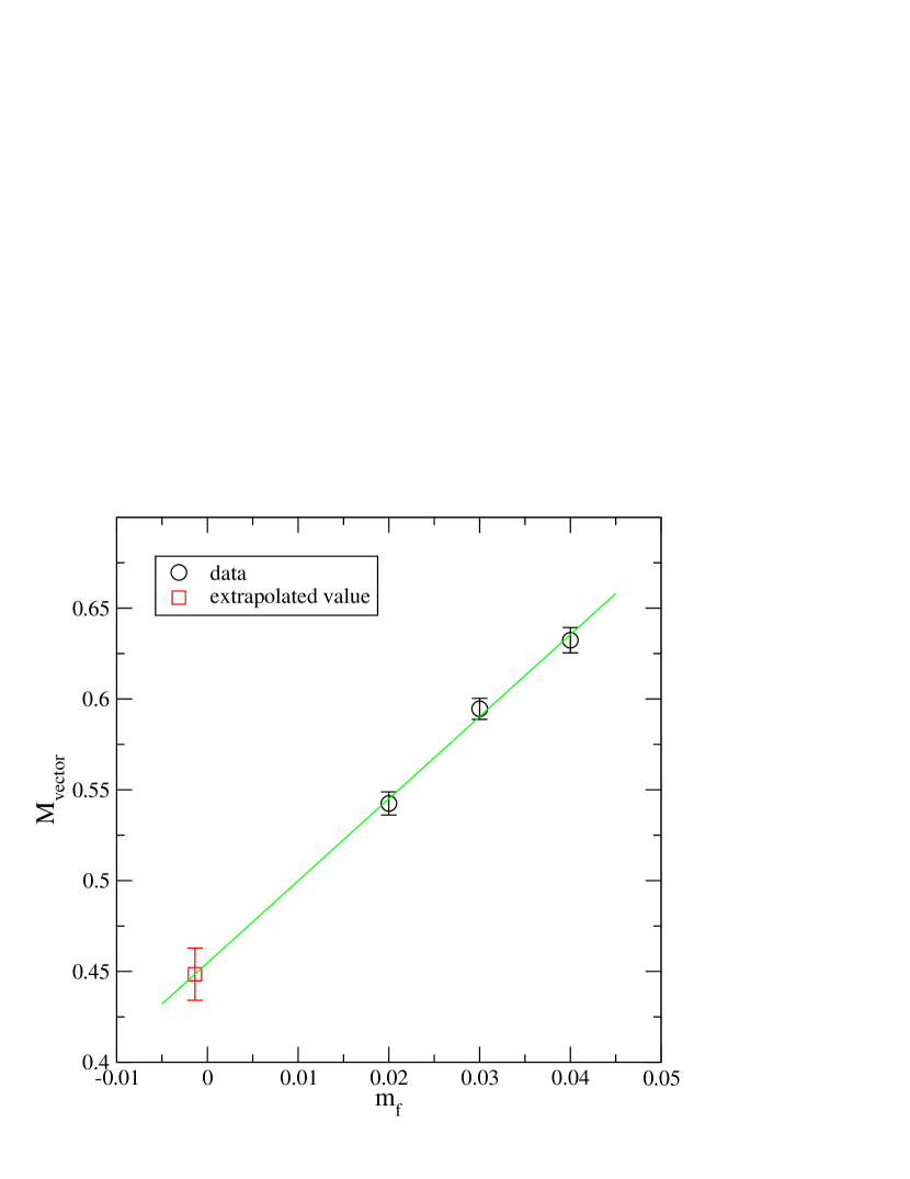
Figure 15: The fitted vector mass in the vector channel for $m_{sea}=m_{val}$. The solid line denotes a linear fit.

References

- Kaplan (1992) D. B. Kaplan, Phys. Lett. B288, 342 (1992), eprint hep-lat/9206013.
- Narayanan and Neuberger (1993) R. Narayanan and H. Neuberger, Phys. Lett. B302, 62 (1993), eprint hep-lat/9212019.
- Shamir (1993) Y. Shamir, Nucl. Phys. B406, 90 (1993), eprint hep-lat/9303005.
- Ginsparg and Wilson (1982) P. H. Ginsparg and K. G. Wilson, Phys. Rev. D25, 2649 (1982).
- Neuberger (1998) H. Neuberger, Phys. Lett. B417, 141 (1998), eprint hep-lat/9707022.
- Blum and Soni (1997a) T. Blum and A. Soni, Phys. Rev. D56, 174 (1997a), eprint hep-lat/9611030.
- Blum and Soni (1997b) T. Blum and A. Soni, Phys. Rev. Lett. 79, 3595 (1997b), eprint hep-lat/9706023.
- Aoki et al. (2000) S. Aoki, T. Izubuchi, Y. Kuramashi, and Y. Taniguchi, Phys. Rev. D62, 094502 (2000), eprint hep-lat/0004003.
- Ali Khan et al. (2001a) A. Ali Khan et al. (CP-PACS), Phys. Rev. D63, 114504 (2001a), eprint hep-lat/0007014.
- Blum et al. (2004) T. Blum et al., Phys. Rev. D69, 074502 (2004), eprint hep-lat/0007038.
- Ali Khan et al. (2001b) A. Ali Khan et al. (CP-PACS), Phys. Rev. D64, 114506 (2001b), eprint [http://arXiv.org/abs]hep-lat/0105020.
- Aoki et al. (2004a) Y. Aoki et al., Phys. Rev. D69, 074504 (2004a), eprint hep-lat/0211023.
- Sasaki et al. (2002) S. Sasaki, T. Blum, and S. Ohta, Phys. Rev. D65, 074503 (2002), eprint hep-lat/0102010.
- Noaki et al. (2003) J. I. Noaki et al. (CP-PACS), Phys. Rev. D68, 014501 (2003), eprint hep-lat/0108013.
- Blum et al. (2003) T. Blum et al. (RBC), Phys. Rev. D68, 114506 (2003), eprint hep-lat/0110075.
- Blum et al. (2002) T. Blum et al., Phys. Rev. D66, 014504 (2002), eprint [http://arXiv.org/abs]hep-lat/0102005.
- Aoki et al. (2004b) S. Aoki et al. (CP-PACS), Phys. Rev. D70, 034503 (2004b), eprint hep-lat/0312011.
- Ali Khan et al. (2002) A. Ali Khan et al. (CP-PACS), Phys. Rev. D65, 054505 (2002), eprint hep-lat/0105015.
- Aoki et al. (2003) S. Aoki et al. (JLQCD), Phys. Rev. D68, 054502 (2003), eprint hep-lat/0212039.
- Kaneko et al. (2004) T. Kaneko et al. (CP-PACS), Nucl. Phys. Proc. Suppl. 129, 188 (2004), eprint hep-lat/0309137.
- Davies et al. (2004) C. T. H. Davies et al. (HPQCD), Phys. Rev. Lett. 92, 022001 (2004), eprint hep-lat/0304004.
- Aubin et al. (2004a) C. Aubin et al. (2004a), eprint hep-lat/0402030.
- Orginos and Toussaint (1999) K. Orginos and D. Toussaint (MILC), Phys. Rev. D59, 014501 (1999), eprint [http://arXiv.org/abs]hep-lat/9805009.
- Orginos et al. (1999) K. Orginos, D. Toussaint, and R. L. Sugar (MILC), Phys. Rev. D60, 054503 (1999), eprint [http://arXiv.org/abs]hep-lat/9903032.
- Lepage (1999) G. P. Lepage, Phys. Rev. D59, 074502 (1999), eprint [http://arXiv.org/abs]hep-lat/9809157.
- Aubin and Bernard (2003a) C. Aubin and C. Bernard, Phys. Rev. D68, 034014 (2003a), eprint hep-lat/0304014.
- Aubin and Bernard (2003b) C. Aubin and C. Bernard, Phys. Rev. D68, 074011 (2003b), eprint hep-lat/0306026.
- Aoki et al. (2002) S. Aoki et al. (JLQCD), Phys. Rev. D65, 094507 (2002), eprint hep-lat/0112051.
- Clark et al. (2003) M. A. Clark, B. Joo, and A. D. Kennedy, Nucl. Phys. Proc. Suppl. 119, 1015 (2003), eprint hep-lat/0209035.
- Clark and Kennedy (2004) M. A. Clark and A. D. Kennedy, Nucl. Phys. Proc. Suppl. 129, 850 (2004), eprint hep-lat/0309084.
- Aoki (1984) S. Aoki, Phys. Rev. D30, 2653 (1984).
- Golterman and Shamir (2003) M. Golterman and Y. Shamir, Phys. Rev. D68, 074501 (2003), eprint hep-lat/0306002.
- Chen et al. (2001) P. Chen et al., Phys. Rev. D64, 014503 (2001), eprint hep-lat/0006010.
- Furman and Shamir (1995) V. Furman and Y. Shamir, Nucl. Phys. B439, 54 (1995), eprint hep-lat/9405004.
- Vranas (1998) P. M. Vranas, Phys. Rev. D57, 1415 (1998), eprint hep-lat/9705023.
- Gottlieb et al. (1987) S. A. Gottlieb, W. Liu, D. Toussaint, R. L. Renken, and R. L. Sugar, Phys. Rev. D35, 2531 (1987).
- Duane et al. (1987) S. Duane, A. D. Kennedy, B. J. Pendleton, and D. Roweth, Phys. Lett. B195, 216 (1987).
- Luscher (1994) M. Luscher, Nucl. Phys. B418, 637 (1994), eprint [http://arXiv.org/abs]hep-lat/9311007.
- Takaishi (2002) T. Takaishi, Phys. Lett. B540, 159 (2002), eprint [http://arXiv.org/abs]hep-lat/0203024.
- Sexton and Weingarten (1992) J. C. Sexton and D. H. Weingarten, Nucl. Phys. B380, 665 (1992).
- Gupta et al. (1990) S. Gupta, A. Irback, F. Karsch, and B. Petersson, Phys. Lett. B242, 437 (1990).
- Christ (2002) N. H. Christ (RBC), Nucl. Phys. Proc. Suppl. 106, 187 (2002).
- Ukawa (2002) A. Ukawa (CP-PACS and JLQCD), Nucl. Phys. Proc. Suppl. 106, 195 (2002).
- Brower et al. (1997) R. C. Brower, T. Ivanenko, A. R. Levi, and K. N. Orginos, Nucl. Phys. B484, 353 (1997), eprint [http://arXiv.org/abs]hep-lat/9509012.
- Horn and Johnson (1986) R. A. Horn and C. R. Johnson, Matrix analysis (Cambridge University Press, 1986), ISBN 0-521-30586-1.
- Takaishi (1996) T. Takaishi, Phys. Rev. D54, 1050 (1996).
- Aoki et al. (2004c) Y. Aoki et al. (RBC) (2004c), in progress.
- Iwasaki (1983a) Y. Iwasaki (1983a), uTHEP-118.
- Iwasaki (1983b) Y. Iwasaki (1983b), uTHEP-117.
- Iwasaki and Yoshie (1984) Y. Iwasaki and T. Yoshie, Phys. Lett. B143, 449 (1984).
- de Forcrand et al. (2000) P. de Forcrand et al. (QCD-TARO), Nucl. Phys. B577, 263 (2000), eprint hep-lat/9911033.
- Ali Khan et al. (2001c) A. Ali Khan et al. (CP-PACS), Phys. Rev. D64, 114501 (2001c), eprint hep-lat/0106010.
- Bilson-Thompson et al. (2003) S. O. Bilson-Thompson, D. B. Leinweber, and A. G. Williams, Ann. Phys. 304, 1 (2003), eprint hep-lat/0203008.
- DeGrand et al. (1998) T. DeGrand, A. Hasenfratz, and T. G. Kovacs, Nucl. Phys. B520, 301 (1998), eprint [http://arXiv.org/abs]hep-lat/9711032.
- Ilgenfritz et al. (2000) E.-M. Ilgenfritz, W. Kerler, M. Muller-Preussker, and H. Stuben (2000), eprint hep-lat/0007039.
- Toussaint (1989) D. Toussaint (1989), from the TASI-89 Summer School, Boulder, Colo., Jun 4-30, 1989.
- Orth et al. (2004) B. Orth, T. Lippert, and K. Schilling, Nucl. Phys. Proc. Suppl. 129, 173 (2004), eprint hep-lat/0309085.
- Orth (2004) B. Orth, Thesis, Univ. Wuppertal WUB-DIS 2004-03 (2004).
- Ali Khan et al. (2004) A. Ali Khan et al. (QCDSF-UKQCD), Nucl. Phys. B689, 175 (2004), eprint hep-lat/0312030.
- Beane (2004a) S. R. Beane, Phys. Rev. D70, 034507 (2004a), eprint hep-lat/0403015.
- Jenkins (1992) E. Jenkins, Nucl. Phys. B368, 190 (1992).
- Leinweber et al. (2000) D. B. Leinweber, A. W. Thomas, K. Tsushima, and S. V. Wright, Phys. Rev. D61, 074502 (2000), eprint hep-lat/9906027.
- Bernard et al. (2004) V. Bernard, T. R. Hemmert, and U.-G. Meissner, Nucl. Phys. A732, 149 (2004), eprint hep-ph/0307115.
- Procura et al. (2004) M. Procura, T. R. Hemmert, and W. Weise, Phys. Rev. D69, 034505 (2004), eprint hep-lat/0309020.
- Beane (2004b) S. R. Beane, Nucl. Phys. B695, 192 (2004b), eprint hep-lat/0403030.
- Bernard and Golterman (1994) C. W. Bernard and M. F. L. Golterman, Phys. Rev. D49, 486 (1994), eprint hep-lat/9306005.
- Golterman and Leung (1998a) M. F. L. Golterman and K.-C. Leung, Phys. Rev. D57, 5703 (1998a), eprint hep-lat/9711033.
- Laiho and Soni (2002) J. Laiho and A. Soni, Phys. Rev. D65, 114020 (2002), eprint [http://arXiv.org/abs]hep-ph/0203106.
- Bernard (2002) C. Bernard (MILC), Phys. Rev. D65, 054031 (2002), eprint hep-lat/0111051.
- Aubin et al. (2004b) C. Aubin et al. (MILC) (2004b), eprint hep-lat/0407028.
- Hashimoto et al. (2003) S. Hashimoto et al. (JLQCD), Nucl. Phys. Proc. Suppl. 119, 332 (2003), eprint hep-lat/0209091.
- Albanese et al. (1987) M. Albanese et al. (APE), Phys. Lett. B192, 163 (1987).
- Bolder et al. (2001) B. Bolder et al., Phys. Rev. D63, 074504 (2001), eprint hep-lat/0005018.
- Luscher and Weisz (1984) M. Luscher and P. Weisz, Nucl. Phys. B240, 349 (1984).
- Necco (2004) S. Necco, Nucl. Phys. B683, 137 (2004), eprint hep-lat/0309017.
- Hashimoto and Izubuchi (2004) K. Hashimoto and T. Izubuchi (RBC) (2004), eprint hep-lat/0409101.
- Iwasaki et al. (1997) Y. Iwasaki, K. Kanaya, T. Kaneko, and T. Yoshie, Phys. Rev. D56, 151 (1997), eprint hep-lat/9610023.
- Michael (1992) C. Michael, Phys. Lett. B283, 103 (1992), eprint hep-lat/9205010.
- Lang and Rebbi (1982) C. B. Lang and C. Rebbi, Phys. Lett. B115, 137 (1982).
- Weisz (1983) P. Weisz, Nucl. Phys. B212, 1 (1983).
- Sommer (1994) R. Sommer, Nucl. Phys. B411, 839 (1994), eprint hep-lat/9310022.
- Hashimoto (2004) K. Hashimoto, In preperation (2004).
- Allton et al. (1999a) C. R. Allton et al. (UKQCD), Phys. Rev. D60, 034507 (1999a), eprint hep-lat/9808016.
- Bali et al. (2000) G. S. Bali et al. (TXL), Phys. Rev. D62, 054503 (2000), eprint hep-lat/0003012.
- Bernard et al. (2000) C. W. Bernard et al., Phys. Rev. D62, 034503 (2000), eprint hep-lat/0002028.
- Allton et al. (1999b) C. R. Allton et al., Phys. Lett. B453, 30 (1999b), eprint hep-lat/9806016.
- Golterman and Leung (1998b) M. F. L. Golterman and K.-C. Leung, Phys. Rev. D57, 5703 (1998b), eprint hep-lat/9711033.
- Izubuchi (2004) T. Izubuchi (RBC), Nucl. Phys. Proc. Suppl. 129, 266 (2004), eprint hep-lat/0310058.
- Ciuchini et al. (1995) M. Ciuchini, E. Franco, G. Martinelli, L. Reina, and L. Silvestrini, Z. Phys. C68, 239 (1995), eprint hep-ph/9501265.
- DeGrand (2004) T. DeGrand (MILC), Phys. Rev. D69, 014504 (2004), eprint hep-lat/0309026.
- Aoki et al. (1998) S. Aoki et al. (JLQCD), Phys. Rev. Lett. 80, 5271 (1998), eprint hep-lat/9710073.
- Garron et al. (2004) N. Garron, L. Giusti, C. Hoelbling, L. Lellouch, and C. Rebbi, Phys. Rev. Lett. 92, 042001 (2004), eprint hep-ph/0306295.
- Bijnens and Prades (1995) J. Bijnens and J. Prades, Nucl. Phys. B444, 523 (1995), eprint hep-ph/9502363.
- Peris and de Rafael (2000) S. Peris and E. de Rafael, Phys. Lett. B490, 213 (2000), eprint hep-ph/0006146.
- Cata and Peris (2003) O. Cata and S. Peris, JHEP 03, 060 (2003), eprint hep-ph/0303162.
- Kilcup (1993) G. Kilcup, Phys. Rev. Lett. 71, 1677 (1993).
- Ishizuka et al. (1993) N. Ishizuka et al., Phys. Rev. Lett. 71, 24 (1993).
- Soni (1996) A. Soni, Nucl. Phys. Proc. Suppl. 47, 43 (1996), eprint hep-lat/9510036.
- Flynn et al. (2004) J. M. Flynn, F. Mescia, and A. S. B. Tariq (UKQCD) (2004), eprint hep-lat/0406013.
- Sharpe (1997) S. R. Sharpe, Nucl. Phys. Proc. Suppl. 53, 181 (1997), eprint hep-lat/9609029.
- Levkova and Mawhinney (2004) L. Levkova and R. Mawhinney, Nucl. Phys. Proc. Suppl. 129, 399 (2004), eprint hep-lat/0309122.