Overlap of the Wilson loop
with the broken-string state

Abstract

Numerical experiments on most gauge theories coupled with matter failed to observe string-breaking effects while measuring Wilson loops only. We show that, under rather mild assumptions, the overlap of the Wilson loop operator with the broken-string state obeys a natural upper bound implying that the signal of string-breaking is in general too weak to be detected by the conventional updating algorithms.

In order to reduce the variance of the Wilson loops in 3-D $\mathbb{Z}_{2}$ gauge Higgs model we use a new algorithm based on the Lüscher-Weisz method combined with a non-local cluster algorithm which allows to follow the decay of rectangular Wilson loops up to values of the order of $10^{-24}$. In this way a sharp signal of string breaking is found.

^a Dipartimento di Fisica Teorica, Università di Torino and
INFN, sezione di Torino, via P. Giuria, 1, I-10125 Torino, Italy.
^b Dipartimento di Fisica, Università di Milano and
INFN, Sezione di Milano, Via Celoria, 16, I-20133 Milano, Italy.

e-mail: gliozzi@to.infn.it, antonio.rago@mi.infn.it
IFUM-793-FT

1 Introduction

The confining force between a pair of static sources in pure gauge theories is mediated by a thin flux tube, or string, joining the two sources. When matter is added to this system the string becomes unstable at large separations and breaks when it reaches a certain length $R_{b}$ to form pairs of matter particles. This breaking should produce the screening of the confining force between the sources and hence the flattening of the static potential.

The lack of any sign of flattening in most systems, while measuring the static potential from Wilson loops only, came as a surprise [1, 2].

One suggestion to arise in literature is that the Wilson loop has a poor overlap with the true ground state, hence the basis of the operators has to be enlarged [3] in order to get a reliable estimate of the potential. Using this multichannel method it has been observed the breaking of the confining string in Higgs models [4] in QCD [5, 6] and in the SU(2) Yang Mills theory with adjoint sources [7]. Even if some cautionary observations have been raised about this method [8], one is led to conclude that the difficulty in observing string breaking with the Wilson loop seems to indicate nothing more than that it has a very small overlap with the broken-string state.

This fact has been directly demonstrated in $2+1~{}d$ SU(2) YM theory with adjoint sources [9] where, using a variance reduction algorithm allowing to detect signals down to $10^{-40}$, it has been clearly observed a rectangular Wilson loop $W(R>R_{b},T)$ changing sharply its slope as a function of $T$ from that associated to the unbroken string (area-law decay) to that of the broken-string state (perimeter-law decay) at a distance much longer than the string breaking scale $R_{b}$. Here we will undertake a similar work for the $2+1~{}d$ $\mathbb{Z}_{2}$ gauge-Higgs model and find a similar result. With the emergence of this long-distance effect a closely related question comes in: why the overlap of the Wilson loop with the broken-string state is so small?.

Before trying to answer to this question, we should mention that do exist gauge systems where such overlap is much bigger. For instance, in the $2+1~{}d$ $\mathbb{Z}_{2}$ gauge-Higgs [10] and in $3+1~{}d$ SU(2) gauge-Higgs models [11] it has been identified a region of the space of the coupling constants where the vacuum has a rather unusual property in that it has, besides the magnetic monopole condensate characterising the confining “phase”, also a non-vanishing electric condensate, like in the dual Higgs phase. We argued [10] that in this region the world sheet of the Wilson loop belongs to the so called tearing phase [12, 13], characterised by the formation of holes of arbitrary large size, reflecting pair creation. As a consequence, larger Wilson loops give rise to larger holes and the vacuum expectation value follows the perimeter-law, signalling string breaking. Actually, measuring Wilson loops in such a special region of the $2+1~{}d~{}\mathbb{Z}_{2}$ gauge Higgs model, we observed [10] a smooth transition from an area decay at relatively short distances to a perimeter decay at long distances.

Hints of an appreciable overlap of large Wilson loops with the broken-string ground state have been also reported in 2+1 dimensional SU(2) gauge theory with two flavours [14] using highly anisotropic improved lattices and even in 3+1 QCD [15], measuring Wilson line correlators in Coulomb gauge with an improved action.

In this paper we consider instead isotropic lattices with standard plaquette action in the confined “phase”. Our main goal is to understand why in these cases, for all coupled gauge systems studied thus far, it is so difficult to observe string breaking using Wilson loops only.

It was argued [13] that in these cases the world sheet associated to the confining string belongs to the normal phase, where the holes induced by dynamical matter have a mean size which does not depend on that of the Wilson loop: larger loops give rise to the formation of more holes. As a consequence they decay with an area-law as in the quenched case. This suggests we assume the following Ansatz for the asymptotic behaviour of large, rectangular Wilson loops

$$W(R,T)\simeq c_{u}\exp[-2\rho(R+T)-\sigma RT]+c_{b}\exp[-2\mu(R+T)]$$ (1)

The first term describes the typical area-law decay of pure Yang-Mills theory with a string tension $\sigma$. The second term is instead the contribution expected in the broken-string state; it decays with a perimeter law controlled by the mass $\mu$ of the so called static-light meson, the lowest bound state of a static source and a dynamical Higgs field or quark .

In [13] it was even conjectured that the perimeter term could be zero (no overlap). Note however that any Wilson loop of finite size receives contributions not only from world sheet configurations typical of the normal phase, but also from those of the tearing phase [16], hence $c_{b}\not=0$.

It is easy to see [9] that for $R<R_{b}$ and $c_{b}$ small enough the first term dominates over the whole range of $T$ and no sign of string-breaking can be seen. When $R>R_{b}$, no matter how small $c_{b}$ is, the above Ansatz implies that at long distances the broken string behaviour eventually prevails, since the first term drops off more rapidly than the second. We must of course also require that the latter should not dominate at distances shorter than the string breaking scale $R_{b}$, thus it is obvious that $c_{b}$ cannot be too big.

A closer look shows (Section 2) that the ratio $c_{b}/c_{u}$ is bounded from above by the following inequality

$$\log\frac{c_{b}}{c_{u}}\leq\,\sigma R_{f}\,(2R_{b}-R_{f})~{}~{},$$ (2)

where $R_{f}$ is the minimal scale of string formation. Inserting this upper bound into (1) one easily checks on the back of an envelope that as $R$ ranges from, say, $R_{b}$ to $2\,R_{b}-R_{f}$, the Wilson loop $W(R,T)$ could deviate from the unbroken string behaviour only for $T\geq 2\,R_{b}-R_{f}$ , where its vacuum expectation value is in general exceedingly small (Section 2).

Thus such a bound gives us a simple explanation of the fact that it is so difficult to see a signal of string breaking while measuring Wilson loop only. It can also be used as a guide to search in the parameter space of the gauge theory a region where it is possible to evaluate the vacuum expectation value of rectangular Wilson loops with $R>R_{b}$ and $T>2\,R_{b}-R_{f}$.

We applied that procedure to the 2+1 dimensional $\mathbb{Z}_{2}$ gauge-Higgs model (Section 3). Although such a system is perhaps the simplest example of a gauge theory coupled to matter in the fundamental representation, the current algorithms are not sufficiently accurate for our purpose. Thus we developed a new one, based on a version of the recent Lüscher-Weisz variance reduction [17] for updating the gauge degrees of freedom, combined with a non-local cluster algorithm for the matter degrees of freedom ( Section 4).

The new algorithm allowed us to detect signals down to $10^{-24}$. We observed in this way rectangular Wilson loops $W(R,T\simeq 2\,R_{b})$ changing abruptly their slope as a function of $R$ as described by the Ansatz (1). It turns out that the breaking point nearly saturates the upper bound (Section 5).

2 The upper bound

Consider a gauge system composed by a gauge field coupled to whatever kind of matter. The confining string between a pair of static sources should be unstable against breaking at large $R$, where dynamical matter particles can materialise to bind to the static sources, forming a pair of bound states called static-light mesons.

Denoting by $\mu$ the mass of the lowest bound state, the static potential is expected to approach the constant value

$$\lim_{R\to\infty}V(R)=2\,\mu~{}~{},$$ (3)

where

$$V(R)=-\lim_{T\to\infty}\frac{1}{T}W(R,T)~{}~{}.$$ (4)

Although Eq (3) refers to an asymptotic value, numerical simulations on these systems show that for all practical purposes we may safely assume

$$V(R)\simeq 2\,\mu~{}~{},~{}~{}~{}~{}R>R_{b}~{}~{}~{},$$ (5)

while in the range $R_{f}\leq R\leq R_{b}$, where the confining string is formed and is stable, the potential should have the typical confining form dictated by the first term of Eq. (1)

$$V(R)\simeq 2\rho+\sigma R~{}~{},~{}~{}~{}R_{f}\leq R\leq R_{b}~{}~{}~{}.$$ (6)

Combining Eq.(5) and (6) yields

$$R_{b}\simeq\frac{2\mu-2\rho}{\sigma}~{}~{}.$$ (7)

Notice that the mass $\mu$ and the perimeter term $\rho$ are not UV finite because of the additive divergent self-energy contributions of the static sources. However, these divergences should cancel in their difference, hence $R_{b}$ is a meaningful physical scale even in the continuum limit.

In the range $R_{f}\leq R\leq R_{b}$, according to Eq.(6), the first term of the Ansatz (1) dominates over the second in the limit $T\to\infty$, hence it should also dominate for any finite $T$, because $V(R)$ is less than $2\,\mu$ in this range of $R$. Thus

$$c_{u}\,e^{-2\rho(R+T)-\sigma RT}\geq c_{b}\,e^{-2\mu(R+T)}~{},~{}R_{f}\leq R\leq R_{b}~{},~{}T>R_{f}~{}.$$ (8)

With the help of Eq.(7), this inequality can eventually be recast into the form

$$\log\frac{c_{b}}{c_{u}}\leq\sigma\,\left[R_{b}(R+T)-RT\right]~{}~{},~{}R_{f}\leq R\leq R_{b},~{}T>R_{f}~{}.$$ (9)

Putting $R=T=R_{f}$ yields the sought after bound (2). For a graphical representation of the Ansatz and the subsequent bounds see Fig. 1.

In the confining string picture, the inequality (8) tells us that a string of length $R_{f}\leq R\leq R_{b}$ is stable and then it can propagate for any interval of $T$. A natural question comes to mind. What happens when we stretch the string beyond $R_{b}$? clearly it becomes unstable against breaking. Let ${\cal T}={\cal T}(R)$ be the amount of “time” it takes for a string of length $R$ to break, defined by the equality of the two terms of the Ansatz (1). Inserting there the upper bound (2) we can find a lower bound for ${\cal T}$ as a function of $R$:

$${\cal T}(R)\geq\frac{R_{b}\,(R-2\,R_{f})+R_{f}^{2}}{R-R_{b}}~{}~{},~{}R>R_{b}~{}.$$ (10)

${\cal T}$ represents the minimal survival time of a string of length $R$ before breaking. In order to maximise the signal one must minimise the area $A(R)=R\,{\cal T}(R)$ of the Wilson loop. Looking at the solution $R_{o}$ of $\frac{d\,A(R)}{d\,R}=0$ one gets after a little algebra

$$T_{b}\equiv{\cal T}(R_{o})=2R_{b}-R_{f}=R_{o}~{}.$$ (11)

It represents the most favourable distance for observing string breaking in the case in which the upper bound were saturated; but even in this limit case the signal is very weak, being proportional to $e^{-\sigma T_{b}^{2}}$. From a computational point of view it is very challenging to reach such length scales in the measure of $W(T,R)$ even in the simplest models. This explains why it is so difficult to see this effect.

Thus far we have neglected the effects due to quantum string fluctuations. A more accurate Ansatz which accounts for these will be used while fitting the numerical data (see Eq.(16)). Had we used such a refined form in deriving the above bounds, we would have obtained much more involved formulae without modifying very much their numerical value.

In deriving the previous inequalities it was assumed that the confining string is created by the Wilson loop. It should be clear that these formulae are not applicable to strings generated by different operators. Notice that different operators correspond to different boundary conditions of the string world sheet and these imply in turn different long distance behaviour. For instance, in the case of a coupled gauge theory at finite temperature, it is quite obvious how to modify the Ansatz (1) in order to describe the Polyakov line correlator (see e.g. Eq.(10) of [13]). In particular the second term is just a constant at any fixed temperature; this implies that the overlap of the Polyakov line correlator with the broken string state is maximal above $R_{b}$, in agreement with the fact that at finite temperature string breaking has been easily seen [20].

3 $\mathbb{Z}_{2}$ gauge-Higgs action and observables

The action of a 2+1 dimensional $\mathbb{Z}_{2}$ gauge theory coupled to Ising matter in a cubic lattice $\Lambda$ can be written as

$$S(\beta_{G},\beta_{I})=-\beta_{I}\sum_{\langle ij\rangle}\varphi_{i}U_{ij}\varphi_{j}-\beta_{G}\sum_{plaq.}U_{\square}~{},$$ (12)

where both the link variable $U_{ij}\equiv U_{\ell}$ and the matter field $\varphi_{i}$ take values $\pm 1$ and $U_{\square}=\prod_{\ell\in\square}U_{\ell}$.

This model is self-dual: the Kramers-Wannier transformation maps the model into itself. Its partition function

$$Z(\beta_{G},\beta_{I})=\int[\mbox{DU]\,[D}\varphi]\,e^{-S(\beta_{G},\beta_{I})}$$ (13)

fulfils the functional equation

$$Z(\beta_{G},\beta_{I})=(\sinh 2\beta_{G}\sinh 2\beta_{I})^{\frac{3}{2}N}Z(\tilde{\beta}_{I},\tilde{\beta}_{G})$$ (14)

with $\tilde{\beta}=-\frac{1}{2}\log(\tanh\beta)$.

The phase diagram of this model was studied long ago [18] and revisited recently[19]. There is an unconfined region surrounded by lines of phase transitions toward the Higgs phase and its dual confining phase. These lines are second order until they are near each other and the self-dual line, where first order transition occurs. Our simulations are of course in the confining phase.

We measured two kinds of observables. The Wilson loop associated to a closed path $C$ of links $\ell$ is defined as usual

$$W(C)=\langle\prod_{l\in C}U_{\ell}\rangle=\frac{1}{Z}\int[\mbox{DU]\,[D}\varphi]\prod_{l\in C}U_{\ell}\,e^{-S}~{}~{}.$$ (15)

We fitted the numerical data using a refinement of the Ansatz (1) which takes into account the universal contribution of the bosonic string quantum fluctuations. Indeed previous numerical work on this subject strongly suggested [16] that the nature of the underlying asymptotic string should be the same as in the pure gauge model [21]. Thus we put

$$W(R,T)\simeq c_{u}\sqrt{\frac{\eta(i)\sqrt{R}}{\eta(\tau)}}\exp[-2\rho(R+T)-\sigma RT]+c_{b}\exp[-2\mu(R+T)]~{},$$ (16)

where $\eta(\tau)$ is the Dedekind function

$$\eta(\tau)=q^{1/24}\,\prod_{n=1}^{\infty}(1-q^{n})~{},~{}q=e^{2i\pi\tau}~{},\tau=i\frac{T}{R}~{}~{}.$$ (17)

We also considered the gauge-invariant propagator $G(T)$ of the static-light meson. It can be constructed by coupling the product of link variables along a line of extent $T$ to the matter fields $\varphi_{0}$ and $\varphi_{T}$ located at both ends

$$G(T)=\langle\varphi_{0}\prod_{\ell\in T}U_{\ell}\,\varphi_{T}\rangle~{}~{}~{}.$$ (18)

When this line is long enough the asymptotic form of its vacuum expectation value is

$$G(T)\simeq c\,e^{-\mu\,T}~{},$$ (19)

and is well suited to measure $\mu$. We did not apply any kind of smearing to the measured operators.

4 The algorithm

The main idea underlying our algorithm relies on the consideration that the Lüscher-Weisz procedure [17], reducing the short wavelength fluctuations, is capable of an error reduction even if we cannot use their argument on the exponential decay of the temporal line correlators, because in presence of interacting matter the confining string breaks.

We proceed as in the Lüscher-Weisz algorithm and split the lattice in sub-lattices formed by temporal slices and evaluate Wilson loops via a stochastic estimate on these sub-lattices. To be specific, consider a rectangular $R\times T$ Wilson loop in the $(x,t)$ plane. Let $U_{0}(x,t)$ $(U_{1}(x,t))$ be the time-like (space-like) link variables. The two spatial sides of length $R$ are associated to the operators ${\mathbb{L}}(0)=\prod_{n=1,R/a}{U}_{1}(n\,a,0)$ and ${\mathbb{L}}(T)=\prod_{n=1,R/a}{U}_{1}(n\,a,T)$ and the operators associated to the two temporal sides are conveniently expressed in terms of pairs of time-like links with the same temporal coordinate $t=n\,a$, which we call ${\mathbb{T}}(R,n\,a)=U_{0}(0,n\,a)U_{0}(R,n\,a)$. We adhere to the notation of Ref.[17], but we need no matrix indices nor complex conjugation, of course. The vacuum expectation value defined in Eq.(15) can be rewritten as

$$W(R,T)=\langle{\mathbb{L}}(0)\prod_{n=1,T/a}{\mathbb{T}}(R,n\,a)\,{\mathbb{L}}(T)\rangle~{}~{}.$$ (20)

Let us split the whole lattice in sub-lattices formed by temporal slices of arbitrary thickness. As observed in ref.[17], owing to the locality of the action, each slice can be analysed independently of the surrounding medium, provided that the link variables of the boundary and the matter field configuration are held fixed.

In the present case the expectation value of the operator ${\mathbb{T}}(R)$ in a time-slice formed by $m$ layers is defined by

$$\begin{split}[{\mathbb{T}}_{\varphi}\{R,j;m\}]\equiv[{\mathbb{T}}(R,j\,a){\mathbb{T}}(R,(j+1)a)\ldots\\ {\mathbb{T}}(R,(j+m-1)a)]=\frac{1}{{\cal Z}_{sub}}\int[\mbox{DU}]\,e^{-S_{sub}[U,\varphi]}\end{split}$$ (21)

where the subscript $sub$ refers to the variables belonging to the sub-lattice.

In our numerical simulations these expectation values are estimated using a heat-bath method for the link variables, alternating in a suitable proportion with a non-local cluster algorithm for updating the matter field $\varphi$ [10].

As in pure gauge case one gets identities like

$$[{\mathbb{T}}_{\varphi}\{R,j;m\}]\,[{\mathbb{T}}_{\varphi}\{R,(j+m);n\}]=[{\mathbb{T}}_{\varphi}\{R,j;m+n\}]~{},$$ (22)

which allow us to rewrite $W(R,T)$ in the form

$$W(R,T)=\langle{\mathbb{L}}(0)\prod_{j=1,T/m\,a}[{\mathbb{T}}_{\varphi}\{R,j;m\}]\;{\mathbb{L}}(T)\rangle~{}~{}.$$ (23)

where for simplicity it is assumed that $T/a$ is a multiple of $m$. In our simulations we chose $m=2$ and $m=3$.

An updating cycle is organised as follow:

1. Generate field configurations of the whole lattice using the heath-bath and the non-local cluster updates as in [10];

2. Hold fixed both the spatial links along some suitably chosen spatial planes and the matter field configuration and update the gauge fields in the interior of the slices to estimate $[{\mathbb{T}}_{\varphi}\{R,j;m\}]$;

3. Combine the stochastic estimates of the previous step with the side operators ${\mathbb{L}}$ of Eq.(23) and update the matter field configurations using the non-local cluster algorithm;

4. Go to 1.

The number $n_{w}$ of updates of the whole lattice (step 1), the number $n_{t}$ of updates inside each time-slice (step 2) and the number $n_{\varphi}$ of updates of the matter field (step 3) are chosen in practice on the basis of a trial and error method in the optimisation process of the error reduction. For instance, in the $m=3$ case one updating cycle was composed of $n_{t}=10^{2}$ gauge updates for each slice followed by one non-local cluster update of the matter configuration (i.e. $n_{\varphi}=1$) and $n_{w}=10^{5}$ gauge updates of the whole lattice. The total number cycles generated to extract our estimates was $4.0\times 10^{4}$. All the simulations for this work were performed on our cluster employing 20 processors for a total amount of 7000 hours each.

5 Results

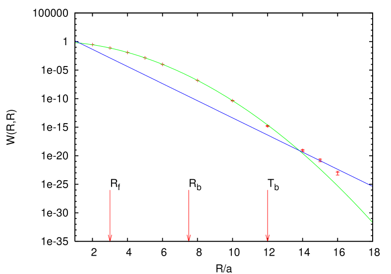
Figure 1: Square Wilson loop versus $R$ in a semilogarithmic plot. The parabolic line is the first term of the Ansatz (16); the straight line represents the contribution of the broken-string state (the second term of the Ansatz) as determined by the fit to rectangular Wilson loops at $T=15\,a$ and large $R$.

We first explored a wide region of the confining phase in order to see whether there exists a parameter range where the lower bound (10) is accessible to realistic simulations. For this purpose we measured the vacuum expectation value of square Wilson loops $W(T,T)$ and the static-light meson correlators $G(T)$ in a wide range of $T$ on a $40^{3}$ cubic lattice in order to estimate the string tension $\sigma$ and the string breaking scale $R_{b}$ trough Eq.(7).

The square Wilson loop data were fitted to the first term of Eq.(16) by progressively eliminating the data of lower $T$ until stable parameters were obtained. While doing this, the scale $R_{f}$ of string formation was determined by picking out the value of $T=R_{f}$ such that the exclusion (inclusion) of $\langle W(R_{f},R_{f})\rangle$ in the fit resulted in a good (bad) $\chi^{2}$ test. In all the cases considered there was no ambiguity in the choice of $R_{f}$, being the corresponding variation of $\chi^{2}$ large enough.

In this way we selected the point $\beta_{G}=0.650$, $\beta_{I}=0.235$ corresponding, in lattice spacing units $a$, to

$$\sigma a^{2}=0.2054(21),~{}\mu a=0.8637(10),~{}R_{f}\simeq 3a,~{}R_{b}\simeq 7.5a,~{}c_{u}=1.19(5)~{}.$$ (24)

Here we concentrated our computational efforts enlarging the lattice size to $50^{3}$ and measuring systematically all the rectangular Wilson loops with $4a\leq R\,\leq 18a$ and $T/a$ a multiple of 2 or 3.

In Fig.2 and Fig.3 we show $W(R,T)$ at $T=15\,a$ and $T=14\,a$ as a function of $R$. Notice the abrupt change in slope, signalling string breaking. The steepest line is not a best fit, but is drawn using the first term of Eq.(16) (unbroken-string term) where the parameters are those fitting the square Wilson loops. The slope of the other line is given by $2\mu$. The only parameter used to fit the data of Fig.2 is $c_{b}$ of Eq.(16). We estimated $c_{b}=43(5)$. This value is used in turn to account for the data of Fig.3. Inserting these values in Eq.(2) we see that the upper bound is nearly saturated and the string-breaking scale in Fig.1 is correspondingly slightly bigger than $T_{b}$.

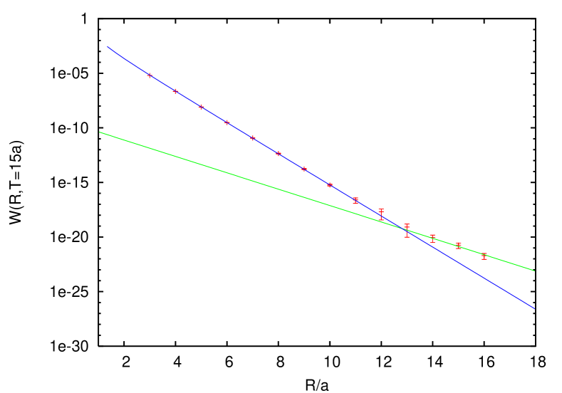
Figure 2: Wilson loop data versus $R$, for $T=15\,a$. The steepest line is not a fit, but represents the first term of Eq.(16) as determined by fitting the square Wilson loops. The slope of the other line is twice the mass of the static-light meson. The only free parameter is the intercept of this line.

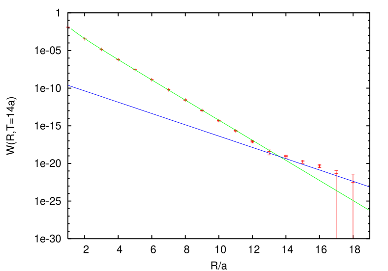
Figure 3: Wilson loop data versus $R$ for $T=14\,a$. We did not fit any parameters but used those of the previous figure combined with the Ansatz (16).

6 Conclusion

The string breaking phenomenon in gauge theories coupled with matter is hardly detectable while measuring Wilson loops only. This reflects the poor overlap of the Wilson loop operator with the broken-string state. A simple way to represent such a behaviour is to assume that the vacuum expectation value of a rectangular Wilson loop $W(R,T)$ is the sum of two terms (see Eq.(1)), one decaying with an area law which prevails at intermediate scales and the other obeying a perimeter law which describes the expected asymptotic behaviour. It is worth noting that the logarithm of the former term is a hyperbola in the $R,T$ plane, while the log of the latter is a straight line; they intersect at two points. One intersection represents the cross over to the broken-string state. The other intersection cannot be completely arbitrary: in order not to spoil the area law at intermediate distances one is forced to put an upper bound of the overlap to the broken-string state of the Wilson operator. Such an upper bound demonstrates a posteriori why it is so difficult to see string breaking in current simulations using Wilson loops only: even if the most favourable conditions were met, namely the saturation of our upper bound and the optimisation of the signal by measuring square Wilson loops, the minimal distance at which string-breaking is visible is $T_{b}=2R_{b}-R_{f}$ (see Eq.(11)), where $R_{b}$ is the string-breaking scale and $R_{f}$ is the minimal scale of string formation. From a computational point of view $T_{b}$ is too large for the current updating algorithms. This explains why earlier studies on Wilson loops in gauge theories coupled to matter, which did not used a variance reduction method, failed to observe string-breaking.

Adapting the Lüscher-Weisz variance reduction method to the 3-D $\mathbb{Z}_{2}$ gauge Higgs model, which is perhaps the simplest gauge theory coupled to matter, we found a clean and beautiful signal of string breaking in the Wilson operator in a region where our upper bound is nearly saturated.

References

- [1] K.D.Born et al., Phys. Lett. b 329 (1994) 325; U.M. Heller eet al., Phys. Lett. B 335 (1994) 71; U. Glässner et al. [SESAM Collaboration], Phys. Lett. B 383 (1996) 98; S. Aoki et al. [CP-PACS Collaboration], Nucl. Phys. B (Proc. Suppl.) 73 (1999) 216; G.S.Bali et al. [TXL Collaboration], Phys. Rev. D 62 (2000) 054503; B.Bolder et al., Phys. Rev. D 63 (2001) 074504.
- [2] G. Poulis and H.D. Trottier, Phys. Lett. B 400 (1997) 358; C. Michael, ArXiv:hep-lat/9809211.
- [3] C. Michael, Nucl Phys. B (Proc. Suppl.) 26 (1992) 417.
- [4] O. Philipsen and H.Wittig, Phys. Rev. Lett. 81 (1998) 4056 [Erratum-ibid.83 (1999) 2684]; F. Knechtli and R. Sommer [ALPHA Collaboration], Phys. Lett. B 440 (1998) 345 and Nucl. Phys. B 590 (2000) 309.
- [5] P.Pennanen and C. Michael, [UKQCD Collaboration], ArXiv:hep-lat/ 0001015 ; C. Bernard et al. [MILC Collaboration], Phys. Rev D 64 (2001) 074509.
- [6] G.S. Bali, Th. Düssel, Th Lippert, H.Neff, Z.Prkçin, K.Schilling, ArXiv:hep-lat/0409137.
- [7] P.W. Stephenson, Nucl. Phys. B 550 (1999) 427; O. Philipsen and H. Wittig, Phys. Lett. B 451 (1999) 146; P. de Forcrand and O.Philipsen, Phys. Lett. B 475 (2000) 280.
- [8] K.Kallio and H.D. Trottier, Phys. Rev. D 66 (2002) 034503.
- [9] S.Kratochvila and P. de Forcrand, Nucl Phys. B 671 (2003) 103.
- [10] F.Gliozzi and A.Rago, Phys. Rev. D 66 (2002) 074511.
- [11] R. Bertle, M. Faber and A. Hirtl, Nucl. Phys. Proc. Suppl. 106 (2002) 664.
- [12] V.A. Kazakov, Phys. Lett. B 237 (1990) 212.
- [13] F.Gliozzi and P. Provero, Nucl. Phys. B 556 (1999) 76; Nucl. Phys. B (Proc. Suppl.) 83 (2000) 461.
- [14] H.D. Trottier, Phys. Rev. D 60 (1999) 034506; H.D. Trottier and K.Y Wong, Nucl. Phys. B (Proc. Suppl.)119 (2003) 673; ArXiv:hep-lat/0408028.
- [15] A.Duncan, E.Eichten and H. Thaker, Phys. Rev D 63 (2001) 111501.
- [16] F. Gliozzi, Nucl. Phys. B (Proc. Suppl.) 94 (2001) 550.
- [17] M. Lüscher and P. Weisz, JHEP 0109 (2001) 010.
- [18] G.Jogeward, J.Stack, Phys.Rev. D 21 (1980) 3360.
- [19] L. Genovese, F.Gliozzi, A.Rago and C. Torrero, Nucl. Phys. ( Proc. Suppl.) 119 (2003) 894.
- [20] E. Laerman, C. DeTar, O. Kaczmarek and F. Karsch, Nucl. Phys. (Proc. Suppl.) 73 (1999) 447.
- [21] M. Caselle, R. Fiore, F. Gliozzi, M. Hasenbusch and P. Provero, Nucl. Phys. B 486 (1997) 245.