Volume dependences from lattice chiral perturbation theory

Abstract

The physics of pions within a finite volume is explored using lattice regularized chiral perturbation theory. This regularization scheme permits a straightforward computational approach to be used in place of analytical continuum techniques. Using the pion mass, decay constant, form factor and charge radius as examples, it is shown how numerical results for volume dependences are obtained at the one-loop level from simple summations.

I Introduction

Lattice QCD is one of the key tools for studying hadronic physics.Wilson It is a numerical technique that employs a finite spatial volume, a finite extent in Euclidean time, and a nonzero spacing between sites on the spacetime lattice. Lattice QCD practitioners also choose unphysically large masses for up and down quarks due to the extreme cost of simulations at their physical values.

The extrapolation to physical up and down quark masses can in principle be performed by using the low energy effective theory for continuum QCD, called chiral perturbation theory (ChPT).GL8485 The Lagrangian of ChPT contains an infinite number of terms, but to a specific order in the small chiral expansion parameters (for the pure pion theory these are $m_{\pi}^{2}/(4\pi f_{\pi})^{2}$ and $p^{2}/(4\pi f_{\pi})^{2}$ with $p$ being a small four-momentum) the number of terms is finite. ChPT has established itself as a valuable formalism for hadronic physics, and its use in connection to lattice QCD is just one important example.

Similarly, the extrapolation in lattice spacing can be discussed within the effective theory for lattice QCD, which is simply ChPT extended to include the effects of the nonzero lattice spacing, $a$. This requires the addition of an infinite number of new terms to the continuum ChPT Lagrangian, each of which is proportional to some positive power of $a$. To a specific order in the lattice spacing expansion, the number of $a$-dependent terms is finite and the numerical values of their coefficients can be determined in principle by matching to a particular definition of lattice QCD. Different lattice QCD Lagrangians (Wilson, Symanzik-improved, etc.) correspond to different lattice ChPT coefficients for the $a$-dependent counterterms. All of these additional terms become irrelevant in the continuum limit.

Lattice ChPT can be defined within a continuum quantum field theory formalism, using (for example) dimensional regularization to handle ultraviolet divergences and retaining the lattice spacing only as prefactor for the $a$-dependent Langrangian counterterms mentioned above.Sharpe ; Bar Another option is to define lattice ChPT in an explicitly discrete spacetime.Rebbi ; ShuSmi ; LO ; BLO The lattice spacing now plays the role of ultraviolet regulator in addition to being the expansion parameter for the $a$-dependent Lagrangian counterterms. With this approach, the lattice spacing appears explicitly in propagators and vertices and also in limits of integration for Feynman loop diagrams. The continuum and discrete methods are essentially equivalent when the inverse lattice spacing lies beyond the regime of ChPT ($1/a>\Lambda_{\chi}\sim m_{\rho}\sim 4\pi f_{\pi}$) as is the case in typical lattice QCD simulations. One method or the other may be preferred for ease of use, or for theoretical discussions of the convergence properties of the ChPT expansion.LO ; BLO

The extrapolation in lattice volume within the framework of ChPT requires in general the inclusion of boundary-valued counterterms to the Lagrangian due to explicit boundary conditions except (as shown by Gasser and LeutwylerGLvolume1 ; GLvolume2 ) for toroidal spacetime. In this case, the only effect of finite volume is the straightforward conversion of loop momentum integrals to loop momentum summations. For a review of recent finite volume ChPT calculations, see Ref. Colangelo . Some of the latest studies in the pion sector are those of Refs. ColDur ; ColHae ; Linetal .

In the present work, we explore the use of lattice regularized ChPT for computing volume dependences. The continuum limit must be identical to any viable continuum regulator, but lattice regularization has the feature of being easy to manage numerically. Beginning from a Lagrangian that displays the lattice spacing explicitly and also maintains exact chiral symmetry,LO one can simply derive the Feynman propagators and vertices then type those directly into a computer program. Loop diagrams are just summations of a finite number of momentum values and the numerics are finite at every step. For a sufficiently small lattice spacing, observables must be independent of $a$.

A brief preliminary discussion of this work can be found in Ref. BLM , but a more detailed study is presented below. Notation for the lattice regularized ChPT Lagrangian is established in Sec. II. The computational method is introduced in Sec. III by examining the two-point pion correlator. This gives the volume dependence of the pion mass, which reproduces a result already known from continuum methods.GLvolume1 ; ColDur The two-point correlator also gives an explicit expression for wave function renormalization in the lattice regularized theory. Section IV contains a computation of volume effects on the pion decay constant which agrees with published continuum calculations.GLvolume1 ; ColHae New results are presented in Sec. V: volume dependences of the pion form factor and the pion charge radius. Section VI mentions some of the challenges that remain to be addressed if lattice regularized ChPT is to be employed for the determination of volume dependences beyond the one-loop level. Appendix A provides an explicit example of calculating Feynman rules from the lattice ChPT action, and Appendix B demonstrates the exact analytic agreement between volume dependences in dimensional regularization and in the continuum limit of lattice regularization.

II A discretized SU(2) chiral Lagrangian

The Lagrangian to be used in this work is an SU(2) version of the SU(3) meson Lagrangian introduced in Ref. LO . Although only a few terms are presently required, here is the complete Lagrangian:

$${\cal L} = {\cal L}_{2}+{\cal L}_{4},$$ (1)

$${\cal L}_{2} = \frac{f^{2}}{4}\left<\nabla^{(+)}_{\mu}U^{\dagger}\nabla^{(+)}_{\mu}U\right>-\frac{f^{2}}{4}\left<\chi^{\dagger}U+\chi U^{\dagger}\right>,$$ (2)

$${\cal L}_{4} = -\frac{1}{4}l_{1}\left<\nabla^{(\pm)}_{\mu}U^{\dagger}\nabla^{(\pm)}_{\mu}U\right>^{2}-\frac{1}{4}l_{2}\left<\nabla^{(\pm)}_{\mu}U^{\dagger}\nabla^{(\pm)}_{\nu}U\right>\left<\nabla^{(\pm)}_{\mu}U^{\dagger}\nabla^{(\pm)}_{\nu}U\right>$$ (3)

$$-\frac{1}{16}(l_{3}+l_{4})\left<\chi^{\dagger}U+\chi U^{\dagger}\right>^{2}+\frac{1}{8}l_{4}\left<\nabla^{(\pm)}_{\mu}U^{\dagger}\nabla^{(\pm)}_{\mu}U\right>\left<\chi^{\dagger}U+\chi U^{\dagger}\right>-l_{5}\left<F_{\mu\nu}^{L}U^{\dagger}F_{\mu\nu}^{R}U\right>$$

$$-\frac{i}{2}l_{6}\left<F_{\mu\nu}^{L}\nabla^{(\pm)}_{\mu}U^{\dagger}\nabla^{(\pm)}_{\nu}U+F_{\mu\nu}^{R}\nabla^{(\pm)}_{\mu}U\nabla^{(\pm)}_{\nu}U^{\dagger}\right>+\frac{1}{16}l_{7}\left<\chi^{\dagger}U-\chi U^{\dagger}\right>^{2}$$

$$-\frac{1}{4}(h_{1}+h_{3}-l_{4})\left<\chi^{\dagger}\chi\right>+\left(2h_{2}+\frac{l_{5}}{2}\right)\left<F_{\mu\nu}^{L}F_{\mu\nu}^{L}+F_{\mu\nu}^{R}F_{\mu\nu}^{R}\right>$$

$$-\frac{1}{16}(h_{1}-h_{3}-l_{4})\left(\left<\chi^{\dagger}U+\chi U^{\dagger}\right>^{2}+\left<\chi^{\dagger}U-\chi U^{\dagger}\right>^{2}-2\left<\chi^{\dagger}U\chi^{\dagger}U+U^{\dagger}\chi U^{\dagger}\chi\right>\right),$$

where $\left<\ldots\right>$ denotes a trace, and summations over repeated Lorentz indices $\mu$ and $\nu$ are understood. $\chi$ is essentially the quark mass matrix,

$$\chi=2B\left(\begin{array}[]{cc}m_{u}&0\\ 0&m_{d}\end{array}\right).$$ (4)

Throughout this work, we restrict ourselves to the isospin limit $m_{u}=m_{d}\equiv m_{q}$. We also choose the exponential representation for pions,

$$U(x)=\exp\left[\frac{i\tau^{a}\pi^{a}(x)}{f}\right],$$ (5)

where $\tau^{a}$ is a Pauli matrix. The external fields are

$$L_{\mu}(x) = \exp\left[-ia\ell_{\mu}(x)\right]=\exp\left[-ia(V_{\mu}(x)-A_{\mu}(x))\right],$$ (6)

$$R_{\mu}(x) = \exp\left[-iar_{\mu}(x)\right]=\exp\left[-ia(V_{\mu}(x)+A_{\mu}(x))\right],$$ (7)

and the corresponding field strength tensors are discretized as follows:

$$4ia^{2}F_{\mu\nu}^{X} = 4-X_{\mu}(x)X_{\nu}(x+a_{\mu})X^{\dagger}_{\mu}(x+a_{\nu})X^{\dagger}_{\nu}(x)$$ (8)

$$-X_{\nu}(x)X^{\dagger}_{\mu}(x-a_{\mu}+a_{\nu})X^{\dagger}_{\nu}(x-a_{\mu})X_{\mu}(x-a_{\mu})$$

$$-X^{\dagger}_{\mu}(x-a_{\mu})X^{\dagger}_{\nu}(x-a_{\mu}-a_{\nu})X_{\mu}(x-a_{\mu}-a_{\nu})X_{\nu}(x-a_{\nu})$$

$$-X^{\dagger}_{\nu}(x-a_{\nu})X_{\mu}(x-a_{\nu})X_{\nu}(x+a_{\mu}-a_{\nu})X^{\dagger}_{\mu}(x)$$

where $X=L,R$. As discussed in Ref. LO , a convenient way to avoid unphysical poles in the spectrum while maintaining invariance under parity is to use a nearest-neighbour derivative in the leading order Lagrangian,

$$\nabla^{(+)}_{\mu}U(x)=\frac{1}{a}\left[R_{\mu}(x)U(x+a_{\mu})L_{\mu}^{\dagger}(x)-U(x)\right],$$ (9)

and a symmetrized derivative at next-to-leading order,

$$\nabla^{(\pm)}_{\mu}U(x)=\frac{1}{2a}\left[R_{\mu}(x)U(x+a_{\mu})L_{\mu}^{\dagger}(x)-R_{\mu}^{\dagger}(x-a_{\mu})U(x-a_{\mu})L_{\mu}(x-a_{\mu})\right].$$ (10)

Notice that the Lagrangian in Eqs. (1-3) contains exactly the same number of terms as the continuum SU(2) ChPT LagrangianGL8485 . As discussed in Sec. I, the most general ChPT Lagrangian would contain extra terms proportional to positive powers of the lattice spacing. Since we are presently interested in volume dependences at the continuum limit, these extra terms are irrelevant and hence omitted for simplicity.

To conclude this section, we recall that the ChPT action is

$$S=a^{4}\sum_{x}{\cal L}(x)-\frac{1}{2}\sum_{x}\left<\ln\left[\frac{2(1-\cos\Phi(x))}{\Phi^{2}(x)}\right]\right>,$$ (11)

where the second term is due to the integration measure.LO For SU(2),

$$\Phi(x)=\frac{-2i}{f}\left(\begin{array}[]{ccc}0&\pi^{3}(x)&-\pi^{2}(x)\\ -\pi^{3}(x)&0&\pi^{1}(x)\\ \pi^{2}(x)&-\pi^{1}(x)&0\end{array}\right).$$ (12)

III The pion mass and wave function renormalization

The Feynman diagrams for the one-loop pion two-point correlator are shown in Fig. 1. To evaluate them within lattice regularization, we choose a hyper-rectangular lattice with lattice spacing $a$ in all four spacetime directions. The lattice is chosen to have $N_{s}$ sites in each of the spatial directions and $N_{t}$ sites in the temporal direction. Our goal is to consider the dependence of observables on spatial volume in the double limit $a\to 0$, $aN_{t}\to\infty$ with $aN_{s}$ held fixed.

Figure 1: Feynman diagrams contributing to the pion two-point correlator at one-loop level in ChPT.

With Feynman vertices obtained from the Lagrangian of Sec. II (see Appendix A for the derivations), the three diagrams of Fig. 1 respectively become

$$\Gamma_{\rm LO} = -x_{\pi}^{2}-\frac{2}{a^{2}}\sum_{\mu}(1-\cos ap_{\mu}),$$ (13)

$$\Gamma_{\rm NLO}^{(a)} = -\frac{2}{3a^{4}f^{2}}-\frac{2x_{\pi}^{4}}{f^{2}}(l_{3}+l_{4})-\frac{2l_{4}x_{\pi}^{2}}{a^{2}f^{2}}\sum_{\mu}\sin^{2}ap_{\mu},$$ (14)

$$\Gamma_{\rm NLO}^{(b)} = \frac{1}{6N_{s}^{3}N_{t}a^{4}f^{2}}\sum_{k}\bigg{(}112+5a^{2}x_{\pi}^{2}-20\sum_{\mu}\cos ap_{\mu}-20\sum_{\mu}\cos ak_{\mu}$$ (15)

$$+12\sum_{\mu}\cos ap_{\mu}\cos ak_{\mu}\bigg{)}D(k),$$

where

$$D(k)=\frac{1}{a^{2}x_{\pi}^{2}+2\sum_{\mu}(1-\cos ak_{\mu})}$$ (16)

is the pion propagator and

$$x_{\pi}=\sqrt{2Bm_{q}}$$ (17)

is the lowest-order pion mass in the continuum limit. The symbol “$\sum_{k}$” in Eq. (15) represents a sum over available lattice 4-momenta; for any function $F$, this means

$$\sum_{k}F(k_{1},k_{2},k_{3},k_{4})\equiv\sum_{n_{1}=1}^{N_{s}}\sum_{n_{2}=1}^{N_{s}}\sum_{n_{3}=1}^{N_{s}}\sum_{n_{4}=1}^{N_{t}}F\left(\frac{2\pi n_{1}}{aN_{s}},\frac{2\pi n_{2}}{aN_{s}},\frac{2\pi n_{3}}{aN_{s}},\frac{2\pi n_{4}}{aN_{t}}\right).$$ (18)

Notice that the middle diagram in Fig. 1 includes the measure contribution as well as the tree-level ${\cal L}_{4}$ contributions.

The pion mass is defined as the energy of a stationary pion. The corresponding expression for the pion mass is the value of $ip_{4}$ which solves $\Gamma=0$ when $\vec{p}=\vec{0}$, where $\Gamma$ is the sum of the three diagrams

$$\Gamma=\Gamma_{\rm LO}+\Gamma_{\rm NLO}^{(a)}+\Gamma_{\rm NLO}^{(b)}.$$ (19)

The result is

$$M_{\pi} = \frac{2}{a}{\rm arcsinh}\left(\frac{aX_{\pi}}{2}\right),$$ (20)

$$X_{\pi}^{2} = x_{\pi}^{2}+\frac{2x_{\pi}^{4}}{f^{2}}l_{3}+x_{\pi}^{2}\sum_{k}\frac{(3-2\cos ak_{4})}{2N_{s}^{3}N_{t}a^{2}f^{2}}D(k)+O(a).$$ (21)

Given numerical values for the Lagrangian parameters $f$, $Bm_{q}$ and $l_{3}$, the pion mass can now be computed directly from Eqs. (20) and (21) for any lattice spacing and volume. As $a\to 0$ the loop diagram diverges and these divergences are cancelled by the $a$ dependence of the bare Lagrangian parameters $f$, $Bm_{q}$ and $l_{3}$. (Since dimensional regularization retains no power divergences, $f$ and $Bm_{q}$ would be scale invariant in that scheme. Lattice regularization does retain power divergences as $a\to 0$ so the parameters $f$ and $Bm_{q}$ do have $a$ dependence in this scheme.) For any $a\neq 0$ the loop diagram is finite, and for sufficiently small $a$ the renormalized pion mass is independent of lattice spacing.

To extract the volume dependence of the pion mass, one needs only the difference of $M_{\pi}$ at two different spatial volumes. The first two diagrams in Fig. 1 cancel in this difference leaving only the loop diagram. As $a\to 0$, the difference between two volumes must be finite because the only available Lagrangian counterterms were in the first two diagrams. The quantities $x_{\pi}$ and $f$ appearing in the loop diagram are the leading chiral-order expressions for the mass and decay constant in the continuum limit. Following Ref. ColDur , we employ $f=86.2$ MeV. One would expect results to become independent of lattice spacing for $a\lesssim 1/(4\pi f_{\pi})\sim 0.2$ fm, and we will choose $N_{t}\gg N_{s}$ so that the temporal direction will not affect our extraction of spatial volume effects in any significant way.

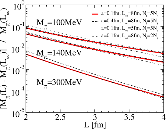
Figure 2: Fractional change in the pion mass as a function of spatial volume.

Figure 2 displays numerical results for the fractional change in the pion mass as a function of spatial volume, relative to the infinite volume pion mass, for $M_{\pi}(L_{\infty})=100$, 140 and 300 MeV, corresponding to $x_{\pi}=100$, 142 and 321 MeV respectively. The computation at “infinite” volume, $L_{\infty}^{3}$, is performed numerically simply by choosing a volume large enough to offer negligible deviations if the volume is increased yet further. Figure 2 shows explicitly the dependence of numerical results on changes to $a$, $L_{\infty}$, and $N_{t}$. As expected, heavier pions have an increased sensitivity to lattice spacing because loop integrals depend on the product $ax_{\pi}$. The computation at $a=0.1$ fm, $L_{\infty}=8$ fm and $N_{t}=5N_{s}$ produces a fractional volume dependence for the pion mass that agrees with the known continuum resultGLvolume1 ; ColDur to within the resolution of this plot for the full range shown, $2~{}{\rm fm}<L<4$ fm. As a confirming cross-check, this known continuum result is derived analytically from our lattice regularized expression in Appendix B.

In addition to the pion mass, Eq. (19) also leads to an expression for the wave function renormalization factor that will be required for all of the observables to be addressed below. Up to irrelevant lattice spacing effects, the two-point correlator can be parametrized as

$$\Gamma = -\left[\tilde{p}^{2}+x_{\pi}^{2}+\Sigma(-\tilde{p}^{2})\right]$$ (22)

$$= -\left[\tilde{p}^{2}+x_{\pi}^{2}+\Sigma(X_{\pi}^{2})+(-\tilde{p}^{2}-X_{\pi}^{2})\Sigma^{\prime}(X_{\pi}^{2})+\delta\Sigma(-\tilde{p}^{2})\right]$$ (23)

where

$$\tilde{p}^{2}=\frac{4}{a^{2}}\sum_{\mu}\sin^{2}\left(\frac{ap_{\mu}}{2}\right),$$ (24)

and $\delta\Sigma(-\tilde{p}^{2})$ vanishes at least as quickly as $(-\tilde{p}^{2}-X_{\pi}^{2})^{2}$ for $-\tilde{p}^{2}\to X_{\pi}^{2}$. The renormalization factor, $Z$, is defined by

$$\Gamma=-\left[\frac{\tilde{p}^{2}+X_{\pi}^{2}}{Z}+\delta\Sigma(-\tilde{p}^{2})\right],$$ (25)

since $X_{\pi}^{2}=x_{\pi}^{2}+\Sigma(X_{\pi}^{2})$ which leads to

$$Z\equiv\frac{1}{1-\Sigma^{\prime}(X_{\pi}^{2})}.$$ (26)

One can read $\Sigma(-\tilde{p}^{2})$ directly from Eqs. (13-15) by choosing $\vec{p}=\vec{0}$, and this gives

$$Z=1-\frac{2x_{\pi}^{2}l_{4}}{f^{2}}+\frac{1}{3N_{s}^{3}N_{t}a^{2}f^{2}}\sum_{k}(5-3\cos ak_{4})D(k)+O(a).$$ (27)

IV The pion decay constant

Figure 3: Feynman diagrams contributing to the pion decay constant at one-loop level in ChPT. A wavy line denotes an axial vector current insertion.

The three Feynman diagrams of Fig. 3 represent the three contributions to the pion decay constant up to one-loop order. Using the vertices and propagators from the Lagrangian in Eqs. (1-3), one finds the following expressions for those three diagrams,

$$G_{\rm LO}\sqrt{Z} = \frac{i\sqrt{2}}{a}f\left[\sin ap_{\mu}+2i\sin^{2}\left(\frac{ap_{\mu}}{2}\right)\right]\sqrt{Z},$$ (28)

$$G_{\rm NLO}^{(a)} = \frac{i2\sqrt{2}}{af}x_{\pi}^{2}l_{4}\exp\left(\frac{iap_{\mu}}{2}\right)\cos\left(\frac{ap_{\mu}}{2}\right)\sin(ap_{\mu}),$$ (29)

$$G_{\rm NLO}^{(b)} = -i\left[\sin ap_{\mu}+2i\sin^{2}\left(\frac{ap_{\mu}}{2}\right)\right]\frac{\sqrt{2}}{3N_{s}^{3}N_{t}a^{3}f}\sum_{k}(7-3\cos ak_{\mu})D(k).$$ (30)

Choosing a stationary pion ($\vec{p}=\vec{0}$) and inserting Eq. (27) for the wave function renormalization factor leads to

$$G_{\rm LO}+G_{\rm NLO}^{(a)}+G_{\rm NLO}^{(b)}=\frac{i\sqrt{2}}{a}f_{\pi}\left[\sin ap_{4}+O(a)\right]$$ (31)

where the one-loop pion decay constant is

$$f_{\pi}=f+\frac{x_{\pi}^{2}l_{4}}{f}-\frac{1}{2N_{s}^{3}N_{t}a^{2}f}\sum_{k}(3-\cos ak_{4})D(k)+O(a).$$ (32)

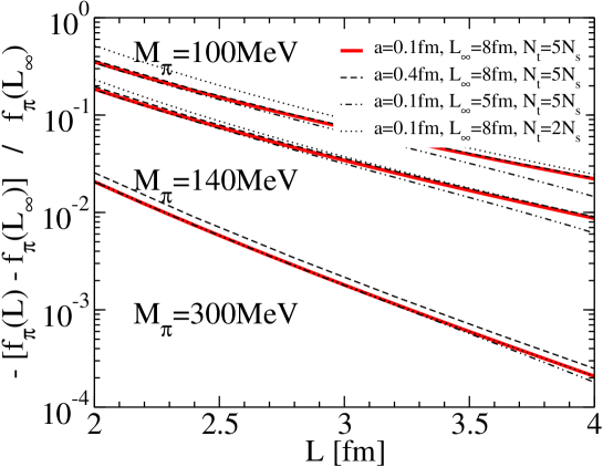
Figure 4: Fractional change in the pion decay constant as a function of spatial volume.

In the difference between $f_{\pi}$ computed from two different lattice volumes, the first two terms in Eq. (32) subtract away. To this chiral order, the remaining parameters $x_{\pi}$ and $f$ can be set to the (infinite volume) physical pion mass and decay constant. The resulting volume dependence of the pion decay constant is displayed in Fig. 4. The magnitude of the volume dependence is similar to that of the pion mass plotted in Fig. 2, but the sign differs — the decay constant is reduced as the volume shrinks, whereas the mass grows with shrinking volume. The computation at $a=0.1$ fm, $L_{\infty}=8$ fm and $N_{t}=5N_{s}$ produces a fractional volume dependence for the pion decay constant that agrees with the known continuum resultGLvolume1 ; ColHae to within the resolution of this plot for the full range shown, $2~{}{\rm fm}<L<4$ fm.

The careful reader will notice that Fig. 4 has a slightly different normalization from the corresponding plot in Ref. BLM ; this difference is higher order in the ChPT expansion, and is due to use of the physical mass and decay constant in Ref. BLM in place of the lowest-order parameters $x_{\pi}$ and $f$. Figures 2 and 4 of the present work show the familiar ratio, $[f_{\pi}(L)/f_{\pi}(L_{\infty})-1]/[M_{\pi}(L)/M_{\pi}(L_{\infty})-1]=-4$, expected from Ref. GLvolume1 .

V The pion form factor and charge radius

The pion electromagnetic form factor is obtained from the Feynman diagrams of Fig. 5, and the charge radius can be extracted from the slope of the form factor at vanishing photon 4-momentum. Using the Lagrangian of Eqs. (1-3), the four diagrams evaluate as follows,

$$H_{\rm LO} = \frac{2Z}{a}\exp\left(\frac{-iaq_{\mu}}{2}\right)\sin a\left(\frac{p+p^{\prime}}{2}\right)_{\mu}$$ (33)

$$H_{\rm NLO}^{(a)} = \frac{2l_{4}x_{\pi}^{2}}{af^{2}}\exp\left(\frac{-iaq_{\mu}}{2}\right)\cos\left(\frac{aq_{\mu}}{2}\right)\sin a(p+p^{\prime})_{\mu}$$ (34)

$$+\frac{2l_{6}}{a^{3}f^{2}}\exp\left(\frac{-iaq_{\mu}}{2}\right)\sum_{\nu}\left[\sin ap_{\mu}\sin ap^{\prime}_{\nu}-\sin ap^{\prime}_{\mu}\sin ap_{\nu}\right]\sin aq_{\nu}\cos\left(\frac{aq_{\mu}}{2}\right),$$

$$H_{\rm NLO}^{(b)} = \frac{-10}{3N_{s}^{3}N_{t}a^{3}f^{2}}\exp\left(\frac{-iaq_{\mu}}{2}\right)\sum_{k}\sin\left(\frac{a(p+p^{\prime})_{\mu}}{2}\right)D(k),$$ (35)

$$H_{\rm NLO}^{(c)} = \frac{4}{N_{s}^{3}N_{t}a^{3}f^{2}}\exp\left(\frac{-iaq_{\mu}}{2}\right)\sum_{k}\sin a(k+q/2)_{\mu}\sum_{\nu}\cos a(p-k)_{\nu}D(k)D(k+q),$$ (36)

where $p$ is the incoming pion momentum, $q$ and $\mu$ are the incoming momentum and Lorentz index of the external photon, and $p^{\prime}\equiv p+q$. The contribution from $H_{\rm NLO}^{(c)}$ can be simplified by removing terms that are odd under interchange of $k$ and $-(k+q)$, since these vanish after summation over $k$. The result is

$$H_{\rm NLO}^{(c)}=\frac{4}{N_{s}^{3}N_{t}a^{3}f^{2}}\exp\left(\frac{-iaq_{\mu}}{2}\right)\sin a\left(\frac{p+p^{\prime}}{2}\right)_{\mu}\sum_{k}\sin^{2}a(k+q/2)_{\mu}D(k)D(k+q).$$ (37)

Figure 5: Feynman diagrams contributing to the pion electromagnetic form factor at one-loop level in ChPT. A wavy line denotes a photon.

The pion form factor, $F(q^{2})$, can be obtained explicitly by choosing $\mu=4$ as follows,

$$H_{\rm LO}+H_{\rm NLO}^{(a)}+H_{\rm NLO}^{(b)}+H_{\rm NLO}^{(c)}=\frac{2}{a}F(q^{2})\exp\left(\frac{-iaq_{4}}{2}\right)\sin a\left(\frac{p+p^{\prime}}{2}\right)_{4}$$ (38)

which gives

$$F(q^{2}) = 1+\frac{l_{6}}{a^{2}f^{2}}\sum_{\nu}\left[\sin ap_{4}\sin ap^{\prime}_{\nu}-\sin ap^{\prime}_{4}\sin ap_{\nu}\right]\sin aq_{\nu}\cos\left(\frac{aq_{4}}{2}\right)$$ (39)

$$-\frac{1}{N_{s}^{3}N_{t}a^{2}f^{2}}\sum_{k}\cos ak_{4}D(k)+\frac{2}{N_{s}^{3}N_{t}a^{2}f^{2}}\sum_{k}\sin^{2}a\left(k+\frac{q}{2}\right)_{4}D(k)D(k+q)$$

$$+O(a).$$

It is interesting to consider the $q\to 0$ limit, since vector current conservation should require $F(0)=1$. From Eq. (39), we see that the term containing $l_{6}$ does vanish in the $q\to 0$ limit. The cancellation at $q=0$ of the two summation terms from Eq. (39) is easily demonstrated in the notation of a temporally infinite lattice,

$$\frac{1}{N_{s}^{3}}\sum_{\vec{k}}\int_{-\pi/a}^{\pi/a}\frac{dk_{4}}{2\pi}\left(2\sin^{2}ak_{4}D^{2}(k)-\cos ak_{4}D(k)\right)$$ (40)

$$= \frac{1}{N_{s}^{3}}\sum_{\vec{k}}\int_{-\pi/a}^{\pi/a}\frac{dk_{4}}{2\pi}\frac{d~{}}{dk_{4}}\left(-\sin ak_{4}D(k)\right)$$

$$= 0.$$

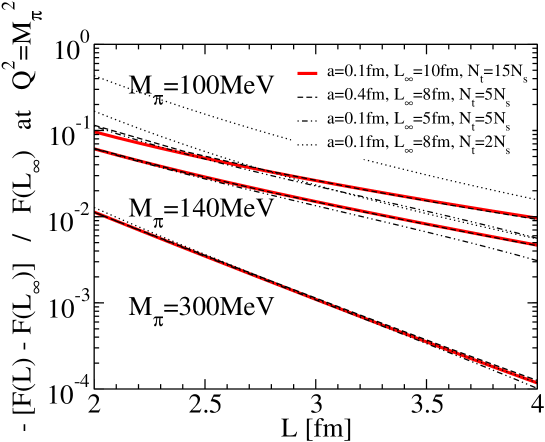
Figure 6: Fractional change in the pion form factor at $Q^{2}=M_{\pi}^{2}$ as a function of spatial volume.

Fig. 6 shows the numerical results for the volume dependence of the pion form factor at $q^{2}=M_{\pi}^{2}$ (meant to represent a typical ChPT mass scale) obtained from Eq. (39), where for numerical ease we work in the Breit frame. As is evident from the plot, the form factor’s fractional volume dependence has a similar magnitude to that obtained for the pion mass and decay constant.

The pion charge radius is extracted from the slope of the form factor at $q^{2}=0$. Choosing $q=(0,0,q_{3},0)$ for definiteness, we find

$$\left<r_{\pi}^{2}\right>_{\pi} = -6\lim_{q^{2}\to 0}\frac{dF(q^{2})}{dq^{2}}$$ (41)

$$= \frac{-6l_{6}}{f^{2}}+\frac{12}{N_{s}^{3}N_{t}f^{2}}\sum_{k}\sin^{2}ak_{4}\left[\cos ak_{3}D^{3}(k)-4\sin^{2}ak_{4}\sin^{2}ak_{3}D^{4}(p)\right]$$

A graph of the fractional volume dependence of this quantity is provided in Fig. 7. The magnitude of the effect is dramatically larger than for the mass, decay constant and form factor simply because the charge radius has (volume-dependent) loop contributions at its first nonzero ChPT order.

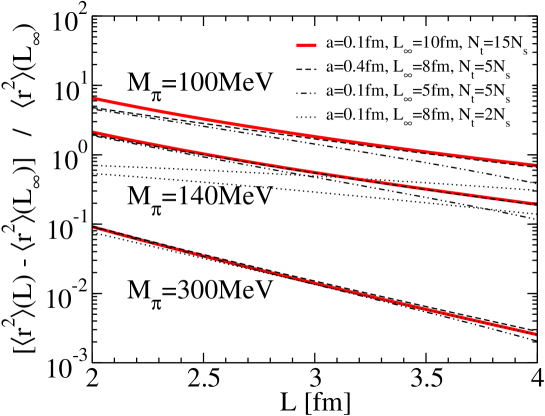
Figure 7: Fractional change in the pion charge radius as a function of spatial volume.

VI Summary and outlook

The pion mass, decay constant, form factor and charge radius have been computed from $O(p^{4})$ chiral perturbation theory in a finite volume by using lattice regularization. A suggested advantage of this regularization scheme is that the renormalization can be carried out numerically, leaving fewer analytical steps to be performed. Explicit expressions for these observables are given as four-dimensional finite sums in Eqs. (21), (32), (39) and (41).

The dimensionally regularized expressions for the pion mass and decay constant are known to be one-dimensional sums over Bessel functionsGLvolume1 ; ColHae , and results from the two regularization schemes agree numerically. In essence, dimensional regularization arrives at a more compact result (i.e. fewer summations) because in that method more of the renormalization is done analytically. Given the small computational cost of the four-dimensional summations, the lattice regularized result is also quite usable in practice. In addition, Appendix B demonstrates that the continuum limit of the lattice regularized result is analytically identical to the dimensional regularized expression, if one chooses to complete the entire analytical calculation instead of the computational scheme proposed in this work.

As emphasized in Ref. Colangelo , it is necessary to extend discussions of volume dependence to the two-loop level, and perhaps beyond, so that the rate of convergence can be explored. In general, two-loop renormalization is substantially more involved than the one-loop case so the reduction of analytical effort obtained by using lattice regularization could be of considerable value. The extension of lattice regularization to two loops will involve the determination of numerical values for the Lagrangian’s low energy constants (and their scale dependences) since they will no longer subtract away in the difference between two volumes. It will also require an understanding of the interplay between power divergences, $1/a^{n}$, and volume dependences, $1/(aN_{s})^{n}$. In particular, one does not want to rely on numerical cancellations among diverging summations. These issues are currently under investigation, in hopes of extending this practical computational method to the domain of multi-loop ChPT calculations.

Appendix A Lattice Feynman rules for the pion mass

This appendix contains an explicit derivation of the Feynman rules required for a one-loop computation of the volume dependence for the pion mass. Only the third diagram of Fig. 1 contributes, which contains the pion propagator and the four pion vertex.

Beginning from Section II and using ellipses to denote terms that do not contribute to the pion two-point function, the relevant terms in the action are

$$\delta S = a^{4}\sum_{x}{\cal L}_{2}(x)+\ldots$$ (42)

$$= -\frac{a^{2}f^{2}}{4}\sum_{x,\mu}{\rm Tr}\left[U^{\dagger}(x+\hat{\mu})U(x)+U^{\dagger}(x)U(x+\hat{\mu})\right]-\frac{a^{4}f^{2}}{2}Bm_{q}\sum_{x}{\rm Tr}\left[U(x)+U^{\dagger}(x)\right]$$

$$+\ldots$$

$$= -a^{2}\delta^{ab}\sum_{x,\mu}\pi^{a}(x)[\pi^{b}(x+\hat{\mu})-\pi^{b}(x)]+\frac{a^{4}x_{\pi}^{2}}{2}\delta^{ab}\sum_{x}\pi^{a}(x)\pi^{b}(x)+\ldots$$

with $\hat{\mu}=a\hat{e}_{\mu}$. This will now be expressed in terms of the Fourier transform,

$$\pi(x)\equiv\frac{1}{N_{s}^{3}N_{t}}\sum_{k}\tilde{\pi}(k)e^{ik\cdot x},$$ (43)

where the summation extends over the set of momenta

$$k=\left(\frac{2\pi n_{1}}{aN_{s}},\frac{2\pi n_{2}}{aN_{s}},\frac{2\pi n_{3}}{aN_{s}},\frac{2\pi n_{4}}{aN_{t}}\right)$$ (44)

with

$$n_{j} = -\frac{N_{s}}{2},-\frac{N_{s}}{2}+1,\ldots,\frac{N_{s}}{2}-1,$$ (45)

$$n_{4} = -\frac{N_{t}}{2},-\frac{N_{t}}{2}+1,\ldots,\frac{N_{t}}{2}-1,$$ (46)

and we have chosen $N_{s},N_{t}$ to be even, in order to keep the presentation simple. Using the relation

$$\sum_{x}e^{ik\cdot x}=N_{s}^{3}N_{t}\delta_{k,0}^{(4)}$$ (47)

leads to

$$\delta S = -\frac{a^{2}\delta^{ab}}{N_{s}^{3}N_{t}}\sum_{k,k^{\prime},\mu}\delta_{k+k^{\prime},0}^{(4)}\tilde{\pi}^{a}(k)\tilde{\pi}^{b}(k^{\prime})\left[e^{ik^{\prime}\cdot\hat{\mu}}-1\right]+\frac{a^{4}x_{\pi}^{2}\delta^{ab}}{2N_{s}^{3}N_{t}}\sum_{k,k^{\prime}}\delta_{k+k^{\prime},0}^{(4)}\tilde{\pi}^{a}(k)\tilde{\pi}^{b}(k^{\prime})+\ldots$$ (48)

$$= \frac{a^{4}\delta^{ab}}{2N_{s}^{3}N_{t}}\sum_{k}\left[x_{\pi}^{2}+\frac{1}{2a^{2}}\sum_{\mu}(1-\cos k\cdot\hat{\mu})\right]\tilde{\pi}^{a}(k)\tilde{\pi}^{b}(-k)+\ldots$$

The Euclidean two-point correlator for incoming pion fields $\tilde{\pi}^{a}(p)$ and $\tilde{\pi}^{b}(q)$ is

$$-\frac{d~{}}{d\left(\frac{\tilde{\pi}^{a}(p)}{N_{s}^{3}N_{t}}\right)}\frac{d~{}}{d\left(\frac{\tilde{\pi}^{b}(q)}{N_{s}^{3}N_{t}}\right)}\left(\frac{\delta S}{a^{4}N_{s}^{3}N_{t}}\right)=-\delta^{ab}\delta_{p+q,0}^{(4)}\left[x_{\pi}^{2}+\frac{2}{a^{2}}\sum_{\mu}(1-\cos p\cdot\hat{\mu})\right].$$ (49)

The pion propagator is the negative inverse of this expression with $p=-q$ and $a=b$, and is $a^{2}D(k)$ of Eq. (16).

To derive the four pion vertex, we again begin from Section II and use ellipses to denote terms that do not contribute,

$$\delta S = a^{4}\sum_{x}{\cal L}_{2}(x)+\ldots$$ (50)

$$= -\frac{a^{2}f^{2}}{4}\sum_{x,\mu}{\rm Tr}\left[U^{\dagger}(x+\hat{\mu})U(x)+U^{\dagger}(x)U(x+\hat{\mu})\right]-\frac{a^{4}f^{2}}{2}Bm_{q}\sum_{x}{\rm Tr}\left[U(x)+U^{\dagger}(x)\right]$$

$$+\ldots$$

$$= -\frac{a^{2}}{48f^{2}}{\rm Tr}(\tau^{a}\tau^{b}\tau^{c}\tau^{d})\sum_{x,\mu}\left[\pi^{a}(x+\hat{\mu})\pi^{b}(x+\hat{\mu})\pi^{c}(x+\hat{\mu})\pi^{d}(x+\hat{\mu})\right.$$

$$-4\pi^{a}(x+\hat{\mu})\pi^{b}(x+\hat{\mu})\pi^{c}(x+\hat{\mu})\pi^{d}(x)+6\pi^{a}(x+\hat{\mu})\pi^{b}(x+\hat{\mu})\pi^{c}(x)\pi^{d}(x)$$

$$\left.-4\pi^{a}(x+\hat{\mu})\pi^{b}(x)\pi^{c}(x)\pi^{d}(x)+\pi^{a}(x)\pi^{b}(x)\pi^{c}(x)\pi^{d}(x)\right]$$

$$-\frac{a^{4}x_{\pi}^{2}}{48f^{2}}{\rm Tr}(\tau^{a}\tau^{b}\tau^{c}\tau^{d})\sum_{x}\pi^{a}(x)\pi^{b}(x)\pi^{c}(x)\pi^{d}(x)+\ldots$$

$$= -\frac{a^{2}}{48f^{2}N_{s}^{12}N_{t}^{4}}{\rm Tr}(\tau^{a}\tau^{b}\tau^{c}\tau^{d})\sum_{x,\mu,k,k^{\prime},k^{\prime\prime},k^{\prime\prime\prime}}\tilde{\pi}^{a}(k)\tilde{\pi}^{b}(k^{\prime})\tilde{\pi}^{c}(k^{\prime\prime})\tilde{\pi}^{d}(k^{\prime\prime\prime})e^{i(k+k^{\prime}+k^{\prime\prime}+k^{\prime\prime\prime})\cdot x}$$

$$\left[e^{i(k+k^{\prime}+k^{\prime\prime}+k^{\prime\prime\prime})\cdot\hat{\mu}}-4e^{i(k+k^{\prime}+k^{\prime\prime})\cdot\hat{\mu}}+6e^{i(k+k^{\prime})\cdot\hat{\mu}}-4e^{ik\cdot\hat{\mu}}+1\right]$$

$$-\frac{a^{4}x_{\pi}^{2}}{48f^{2}N_{s}^{12}N_{t}^{4}}{\rm Tr}(\tau^{a}\tau^{b}\tau^{c}\tau^{d})\sum_{x,k,k^{\prime},k^{\prime\prime},k^{\prime\prime\prime}}\tilde{\pi}^{a}(k)\tilde{\pi}^{b}(k^{\prime})\tilde{\pi}^{c}(k^{\prime\prime})\tilde{\pi}^{d}(k^{\prime\prime\prime})e^{i(k+k^{\prime}+k^{\prime\prime}+k^{\prime\prime\prime})\cdot x}$$

$$= -\frac{a^{2}}{24f^{2}N_{s}^{9}N_{t}^{3}}{\rm Tr}(\tau^{a}\tau^{b}\tau^{c}\tau^{d})\sum_{k,k^{\prime},k^{\prime\prime}}\tilde{\pi}^{a}(k)\tilde{\pi}^{b}(k^{\prime})\tilde{\pi}^{c}(k^{\prime\prime})\tilde{\pi}^{d}(-k-k^{\prime}-k^{\prime\prime})$$

$$\left[2a^{2}x_{\pi}^{2}+\sum_{\mu}\left(1-2e^{ik\cdot\hat{\mu}}-3e^{i(k+k^{\prime})\cdot\hat{\mu}}-2e^{i(k+k^{\prime}+k^{\prime\prime})\cdot\hat{\mu}}\right)\right].$$

The Euclidean four-point correlator (i.e. the Feynman rule) for incoming pion fields $\tilde{\pi}^{a}(p)$, $\tilde{\pi}^{b}(q)$, $\tilde{\pi}^{c}(r)$ and $\tilde{\pi}^{d}(-p-q-r)$ is

$$-\frac{d~{}}{d\left(\frac{\tilde{\pi}^{a}(p)}{N_{s}^{3}N_{t}}\right)}\frac{d~{}}{d\left(\frac{\tilde{\pi}^{b}(q)}{N_{s}^{3}N_{t}}\right)}\frac{d~{}}{d\left(\frac{\tilde{\pi}^{c}(r)}{N_{s}^{3}N_{t}}\right)}\frac{d~{}}{d\left(\frac{\tilde{\pi}^{d}(-p-q-r)}{N_{s}^{3}N_{t}}\right)}\left(\frac{\delta S}{a^{4}N_{s}^{3}N_{t}}\right)$$ (51)

$$= \frac{2}{3a^{2}f^{2}}\left(\delta^{ab}\delta^{cd}+\delta^{ac}\delta^{bd}+\delta^{ad}\delta^{bc}\right)\sum_{\mu}\left(1-\cos p_{\mu}-\cos q_{\mu}-\cos r_{\mu}-\cos(p+q+r)_{\mu}\right)$$

$$+\frac{x_{\pi}^{2}}{3f^{2}}\left(\delta^{ab}\delta^{cd}+\delta^{ac}\delta^{bd}+\delta^{ad}\delta^{bc}\right)+\frac{2}{a^{2}f^{2}}\delta^{ab}\delta^{cd}\sum_{\mu}\cos(p+q)_{\mu}$$

$$+\frac{2}{a^{2}f^{2}}\delta^{ac}\delta^{bd}\sum_{\mu}\cos(p+r)_{\mu}+\frac{2}{a^{2}f^{2}}\delta^{ad}\delta^{bc}\sum_{\mu}\cos(q+r)_{\mu}.$$

The $a\to 0$ limit reproduces the standard continuum Feynman rule as expected.

Appendix B Analytic derivation of the continuum limit

In the main body of this article, lattice regularized results were left in the form of loop summations over products of Feynman rules, since this is sufficient to produce numerical results. As expected, the numerics agreed with analytic dimensional regularized calculations where available, since physics does not depend on regularization scheme. Using the volume dependence of the pion mass as an explicit example, this appendix verifies that continuing the analytic steps in the lattice regularization approach, and taking the continuum limit, leads to the same analytic result that comes from dimensional regularization.

From Eqs. (20) and (21), lattice regularization produces the following difference in pion mass for two lattice volumes,

$$\left[M_{\pi}(L)-M_{\pi}(L^{\prime})\right]_{{\rm finite~{}}a} = \lim_{N_{t}\to\infty}\left[\frac{x_{\pi}}{4a^{2}f^{2}N_{s}^{3}N_{t}}\sum_{k}\frac{3-2\cos ak_{4}}{a^{2}x_{\pi}^{2}+2\sum_{\mu}(1-\cos ak_{\mu})}\right.$$ (52)

$$\left.-\frac{x_{\pi}}{4a^{2}f^{2}(N_{s}^{\prime})^{3}N_{t}}\sum_{k^{\prime}}\frac{3-2\cos ak_{4}}{a^{2}x_{\pi}^{2}+2\sum_{\mu}(1-\cos ak_{\mu}^{\prime})}\right]+O(a),\quad$$

where the summations extend over the set of momenta

$$k=\left(\frac{2\pi n_{1}}{aN_{s}},\frac{2\pi n_{2}}{aN_{s}},\frac{2\pi n_{3}}{aN_{s}},\frac{2\pi n_{4}}{aN_{t}}\right),~{}~{}~{}k^{\prime}=\left(\frac{2\pi n_{1}^{\prime}}{aN_{s}^{\prime}},\frac{2\pi n_{2}^{\prime}}{aN_{s}^{\prime}},\frac{2\pi n_{3}^{\prime}}{aN_{s}^{\prime}},\frac{2\pi n_{4}}{aN_{t}}\right),$$ (53)

with

$$n_{j} = -\frac{N_{s}}{2},-\frac{N_{s}}{2}+1,\ldots,\frac{N_{s}}{2}-1,$$ (54)

$$n_{j}^{\prime} = -\frac{N_{s}^{\prime}}{2},-\frac{N_{s}^{\prime}}{2}+1,\ldots,\frac{N_{s}^{\prime}}{2}-1,$$ (55)

$$n_{4} = -\frac{N_{t}}{2},-\frac{N_{t}}{2}+1,\ldots,\frac{N_{t}}{2}-1$$ (56)

and $N_{s},N^{\prime}_{s},N_{t},N^{\prime}_{t}$ even.

Using a double angle formula from basic trigonometry, Eq. (52) can be re-expressed as

$$\left[M_{\pi}(L)-M_{\pi}(L^{\prime})\right]_{{\rm finite~{}}a} = \lim_{N_{t}\to\infty}\left[\frac{x_{\pi}}{4a^{2}f^{2}N_{s}^{3}N_{t}}\sum_{k}\frac{1+4\sin^{2}(ak_{4}/2)}{a^{2}x_{\pi}^{2}+4\sum_{\mu}\sin^{2}(ak_{\mu}/2)}\right.$$ (57)

$$\left.-\frac{x_{\pi}}{4a^{2}f^{2}(N_{s}^{\prime})^{3}N_{t}}\sum_{k^{\prime}}\frac{1+4\sin^{2}(ak_{4}^{\prime}/2)}{a^{2}x_{\pi}^{2}+4\sum_{\mu}\sin^{2}(ak_{\mu}^{\prime}/2)}\right]+O(a).$$

Since this mass difference is finite even in the continuum limit, and since the Taylor expansion of $\sin\theta$ satisfies absolute convergence term by term over the entire range of interest, $-\pi/2\leq\theta\leq\pi/2$, the leading volume dependence is obtained by retaining the leading term in this Taylor expansion. The result is

$$\left[M_{\pi}(L)-M_{\pi}(L^{\prime})\right]_{{\rm finite~{}}a} = \frac{x_{\pi}}{4a^{4}f^{2}}\lim_{N_{t}\to\infty}\left[\frac{1}{N_{s}^{3}N_{t}}\sum_{k}\frac{1}{x_{\pi}^{2}+\sum_{\mu}k_{\mu}^{2}}-\frac{1}{(N_{s}^{\prime})^{3}N_{t}}\sum_{k^{\prime}}\frac{1}{x_{\pi}^{2}+\sum_{\mu}k_{\mu}^{\prime}}\right]$$ (58)

$$+O(a).$$

As stated in Sec. III, our goal is to consider the dependence of observables on spatial volume in the double limit $a\to 0$, $T\equiv aN_{t}\to\infty$ with $L\equiv aN_{s}$ (and for now $L^{\prime}\equiv aN_{s}^{\prime}$ also) held fixed. With this simple change of variables (but leaving $a$ finite momentarily), we obtain

$$\left[M_{\pi}(L)-M_{\pi}(L^{\prime})\right]_{{\rm finite~{}}a} = \frac{x_{\pi}}{4f^{2}}\lim_{T\to\infty}\left[\frac{1}{L^{3}T}\sum_{n}\frac{1}{x_{\pi}^{2}+\sum_{j}(2\pi n_{j}/L)^{2}+(2\pi n_{4}/T)^{2}}\right.$$ (59)

$$\left.-\frac{1}{(L^{\prime})^{3}T}\sum_{n^{\prime}}\frac{1}{x_{\pi}^{2}+\sum_{j}(2\pi n_{j}^{\prime}/L^{\prime})^{2}+(2\pi n_{4}/T)^{2}}\right]+O(a)$$

$$= \frac{x_{\pi}}{4f^{2}}\int_{-\pi/a}^{\pi/a}\frac{dp_{4}}{2\pi}\left[\frac{1}{L^{3}}\sum_{\vec{n}}\frac{1}{x_{\pi}^{2}+\sum_{j}(2\pi n_{j}/L)^{2}+p_{4}^{2}}\right.$$

$$\left.-\frac{1}{(L^{\prime})^{3}}\sum_{\vec{n}^{\prime}}\frac{1}{x_{\pi}^{2}+\sum_{j}(2\pi n_{j}^{\prime}/L^{\prime})^{2}+p_{4}^{2}}\right]+O(a).$$

We now take the continuum limit, which merely extends the bounds of summation and integration to $\pm\infty$. The integral over $p_{4}$ can be performed in closed form,

$$M_{\pi}(L)-M_{\pi}(L^{\prime}) = \frac{x_{\pi}}{8f^{2}}\left[\frac{1}{L^{3}}\sum_{\vec{n}}\frac{1}{\sqrt{x_{\pi}^{2}+\sum_{j}(2\pi n_{j}/L)^{2}}}-\frac{1}{(L^{\prime})^{3}}\sum_{\vec{n}^{\prime}}\frac{1}{\sqrt{x_{\pi}^{2}+\sum_{j}(2\pi n_{j}^{\prime}/L^{\prime})^{2}}}\right]$$

$$= \frac{x_{\pi}}{8f^{2}\sqrt{\pi}}\int_{0}^{\infty}{ds}\frac{e^{-sx_{\pi}^{2}}}{\sqrt{s}}\left[\frac{1}{L^{3}}\sum_{\vec{n}}e^{-s\sum_{j}(2\pi n_{j}/L)^{2}}-\frac{1}{(L^{\prime})^{3}}\sum_{\vec{n}^{\prime}}e^{-s\sum_{j}(2\pi n_{j}^{\prime}/L^{\prime})^{2}}\right].$$

Letting $L^{\prime}\to\infty$ gives

$$M_{\pi}(L)-M_{\pi} = \frac{x_{\pi}}{8f^{2}\sqrt{\pi}}\int_{0}^{\infty}{ds}\frac{e^{-sx_{\pi}^{2}}}{\sqrt{s}}\left[\frac{1}{L^{3}}\sum_{\vec{n}}e^{-s\sum_{j}(2\pi n_{j}/L)^{2}}-\int_{-\infty}^{\infty}\frac{d^{3}p}{(2\pi)^{3}}e^{-s\vec{p}^{2}}\right]$$ (61)

$$= \frac{x_{\pi}}{8f^{2}\sqrt{\pi}}\int_{0}^{\infty}{ds}\frac{e^{-sx_{\pi}^{2}}}{\sqrt{s}}\left[\frac{1}{L^{3}}\sum_{\vec{n}}e^{-s\sum_{j}(2\pi n_{j}/L)^{2}}-\frac{1}{(4\pi s)^{3/2}}\right],$$

where $M_{\pi}\equiv M_{\pi}(\infty)$. We can now make use of a relation that appears in Ref. BecVil ,

$$\sum_{n=-\infty}^{\infty}e^{-\tau n^{2}}=\sqrt{\frac{\pi}{\tau}}\sum_{n=-\infty}^{\infty}e^{-\pi^{2}n^{2}/\tau},$$ (62)

to obtain

$$M_{\pi}(L)-M_{\pi} = \frac{x_{\pi}}{64f^{2}\pi^{2}}\int_{0}^{\infty}{ds}\frac{e^{-sx_{\pi}^{2}}}{s^{2}}\left[\sum_{\vec{n}}e^{-\vec{n}^{2}L^{2}/(4s)}-1\right]$$ (63)

$$= \frac{x_{\pi}}{64f^{2}\pi^{2}}\int_{0}^{\infty}{ds}\frac{e^{-sx_{\pi}^{2}}}{s^{2}}\sum_{\vec{n}\neq\vec{0}}e^{-\vec{n}^{2}L^{2}/(4s)}$$

$$= \frac{x_{\pi}^{2}}{16f^{2}\pi^{2}L}\sum_{\vec{n}\neq\vec{0}}\frac{K_{1}(x_{\pi}L\sqrt{n_{1}^{2}+n_{2}^{2}+n_{3}^{2}})}{\sqrt{n_{1}^{2}+n_{2}^{2}+n_{3}^{2}}},$$

where $K_{1}(x)$ is a Bessel function of the second kind. This is the result known from dimensional regularized calculations.GLvolume1 ; ColDur Though expressed as a triple summation over $n_{1}$, $n_{2}$ and $n_{3}$, the function only contains the sum of squares, $n_{1}^{2}+n_{2}^{2}+n_{3}^{2}$, thus allowing $M_{\pi}(L)-M_{\pi}$ to be represented by a one-dimensional summation when multiplicity factors are defined.ColDur

References

- (1) K. G. Wilson, Phys. Rev. D 10, 2445 (1974).
- (2) J. Gasser and H. Leutwyler, Ann. Phys. 158, 142 (1984); J. Gasser and H. Leutwyler, Nucl. Phys. B 250, 465 (1985).
- (3) S. R. Sharpe and R. J. Singleton, Phys. Rev. D 58, 074501 (1998); W. J. Lee and S. R. Sharpe, Phys. Rev. D 60, 114503 (1999).
- (4) For a recent review, see O. Bär, hep-lat/0409123.
- (5) S. Myint and C. Rebbi, Nucl. Phys. B 421, 241 (1994); A. R. Levi, V. Lubicz and C. Rebbi, Phys. Rev. D 56, 1101 (1997).
- (6) I. A. Shushpanov and A. V. Smilga, Phys. Rev. D 59, 054013 (1999).
- (7) R. Lewis and P. P. A. Ouimet, Phys. Rev. D 64, 034005 (2001).
- (8) B. Borasoy, R. Lewis and P. P. A. Ouimet, Phys. Rev. D 65, 114023 (2002); B. Borasoy, R. Lewis and P. P. A. Ouimet, Nucl. Phys. (Proc.Suppl.) 128, 141 (2004).
- (9) J. Gasser and H. Leutwyler, Phys. Lett. B 184, 83 (1987).
- (10) J. Gasser and H. Leutwyler, Nucl. Phys. B 307, 763 (1988).
- (11) G. Colangelo, hep-lat/0409111.
- (12) G. Colangelo and S. Dürr, Eur. Phys. J. C 33, 543 (2004);
- (13) G. Colangelo and C. Haefeli, Phys. Lett. B 590, 258 (2004);
- (14) C.-J. D. Lin, G. Martinelli, E. Pallante, C. T. Sachrajda and G. Villadoro, Phys. Lett. B 581, 207 (2004).
- (15) B. Borasoy, R. Lewis and D. Mazur, hep-lat/0408040.
- (16) D. Bećirević and G. Villadoro, Phys. Rev. D 69, 054010 (2004).