The dual Meissner effect in SU(2) Landau gauge

Abstract

The dual Meissner effect is observed without monopoles in quenched $SU(2)$ QCD with Landau gauge-fixing. Abelian as well as non-Abelian electric fields are squeezed. Magnetic displacement currents which are time-dependent Abelian magnetic fields play a role of solenoidal currents squeezing Abelian electric fields. Monopoles are not always necessary to the dual Meissner effect. The squeezing of the electric flux means the dual London equation and the massiveness of the Abelian electric fields as an asymptotic field. The mass generation of the Abelian electric fields is related to a gluon condensate $<A^{a}_{\mu}A^{a}_{\mu}>\neq 0$ of mass dimension 2.

1 Introduction

To understand color confinement mechanism is still an unsolved important problem. The dual Meissner effect is believed to be the mechanismtHooft:1975pu ; Mandelstam:1974pi . However what causes the dual Meissner effect is not clarified. A possible candidate is magnetic monopoles which appear after projecting $SU(3)$ QCD to an Abelian $U(1)^{2}$ theory by a partial gauge fixingtHooft:1981ht . If such monopoles condense, color confinement could be understood due to the dual Meissner effect. Actually an Abelian projection adopting a special gauge called Maximally Abelian gauge (MA)suzuki-83 ; kronfeld leads us to interesting resultsAbelianDominance ; Reviews which support the idea of monopoles after an Abelian projection. See Fig.1 in which the dual Meissner effect due to monopole currents as a solenoidal current is seen beautifullyKoma:2003gq .

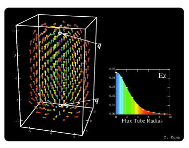
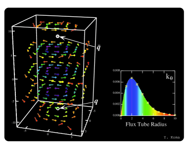
Figure 1: Abelian electric field flux and monopole currents in MA gaugeKoma:2003gq .

Now a natural question arises. What happens in other general Abelian projections or even without any Abelian projection? For example, consider an Abelian projection diagonalizing Polyakov loops. Monopoles exist in the continuum limit at a point where eigenvalues of Polyakov loops are degeneratetHooft:1981ht . But it is easy to show that such a point runs only in the time-like direction. This means only time-like monopoles which do not contribute to the string tension exist in the Abelian projectionmaxim . Discuss another simple case of Landau gauge. There vacuum configurations are so smooth and it is easy to check numerically that no monopoles coming from singularities exist. Without space-like monopoles or monopoles themselves, monopole condensation could not occur. We have to find another confinement mechanism.

In this note, we show that the dual Meissner effect in an Abelian sense works good even when monopoles do not exist, performing Monte-Carlo simulations of quenched $SU(2)$ QCD with Landau gauge fixing. Instead of monopoles, time-dependent Abelian magnetic fields regarded as magnetic displacement currents are squeezing Abelian electric fields. The dual Meissner effect leads us to the dual London equation and the mass generation of the Abelian electric fields which suggests the existence of a dimension 2 gluon condensate. Our present numerical results are not perfect, since the continuum limit, the infinite-volume limit and the gauge-independence are not studied yet. Moreover our discussions use Abelian components only on the basis of not yet clarified assumption that Abelian components are dominant in the infrared QCD (Abelian dominanceAbelianDominance ; Reviews ; greensite-96 ; Cea:1995zt ). Nevertheless authors think the present results are very interesting to general readers, since they show for the first time the Abelian dual Meissner effect is working in lattice non-Abelian QCD without resorting to monopoles coming from a singular gauge transformationfaber . The gauge adopted here is the simplest one only to get smooth configurations. The present results hence suggest the Abelian dual Meissner effect is the real universal mechanism of color confinement which has been sought for many years. Moreover the relation of the Abelian dual Meissner effect with the dimension 2 gluon condensate sheds new light on the importance of the gluon condensate zakharov ; kondo ; dudal ; arriola ; slavnov . Detailed studies, a direct proof of Abelian dominance and extensions to $SU(3)$ and full QCD in zero and finite-temperature cases are in progress.

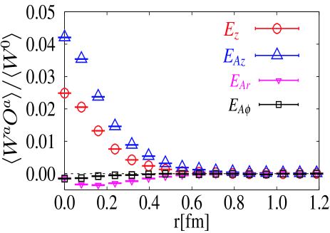
Figure 2: Abelian $\vec{E}_{A}$ and non-Abelian $\vec{E}$ electric field profiles in Landau gauge. $W(R\times T=6\times 6)$ is used.

2 Simulation details

As a lattice quenched $SU(2)$ QCD, we use an improved gluonic action found by Iwasakiiwasaki .

$$S=\beta\left\{c_{0}\sum Tr(plaquette)+c_{1}\sum Tr(rectangular)\right\},$$ (1)

with which better scaling behaviors of physical quantities are expected. The mixing parameters are fixed as $c_{0}+8c_{1}=1$ and $c_{1}=-0.331$.

To measure correlations of gauge-variant electric and magnetic fields directly, we adopt a simplest gauge called Landau gauge which maximizes $\sum_{s,\mu}Tr[U_{\mu}(s)+U_{\mu}^{\dagger}(s)]$. After the gauge fixing, we try to measure electric and magnetic flux distributions by evaluating correlations of Wilson loops and field strengths. For comparison, we also use MA gauge where $\sum_{s,\mu}Tr[U_{\mu}(s)\sigma_{3}U_{\mu}^{\dagger}(s)\sigma_{3}]$ is maximized. To get a good signal to noise ratio, the APE smearing techniqueAPE is used when evaluating Wilson loops $W(R,T)=W^{0}+iW^{a}\sigma^{a}$:

$$U_{i}(s)\longrightarrow N\left\{U_{i}(s)+\alpha\sum_{j\neq i}U_{j}(s)U_{i}(s+\hat{j})U_{j}^{\dagger}(n+\hat{i})\right\},$$ (2)

where $N$ is normalization factor and $\alpha$ is a free parameter. We have used $\alpha=0.2$ and $N=80$.

Measurements of the string tension make us fix the scale when we use $\sqrt{\sigma}=440$MeV. We adopt a coupling constant $\beta=1.2$ in which the lattice distance $a(\beta=1.2)$ is $0.07921(22)$[fm]. The scale is chosen only because we compare our results with those studied extensively in MA gaugebali-96 ; Koma:2003gq . The lattice size is $32^{4}$ and after 5000 thermalization, we have prepared 5000 thermalized configurations per each 100 sweeps for measurements.

Non-Abelian electric and magnetic fields are defined from $1\times 1$ plaquette $U_{\mu\nu}(s)=U^{0}_{\mu\nu}+iU^{a}_{\mu\nu}\sigma^{a}$ as done in Ref.bali-94 :

$$E^{a}_{k}(s) \equiv \frac{1}{2}(U^{a}_{4k}(s-\hat{k})+U^{a}_{4k}(s))$$

$$B^{a}_{k}(s) \equiv \frac{1}{8}\epsilon_{klm}(U_{lm}^{a}(s-\hat{l}-\hat{m})$$

$$+U_{lm}^{a}(s-\hat{l})+U_{lm}^{a}(s-\hat{m})+U_{lm}^{a}(s))$$

We also define Abelian electric ($E_{Ai}^{a}$) and magnetic fields ($B_{Ai}^{a}$) similarly using Abelian plaquettes $\theta_{\mu\nu}^{a}(s)$ defined through link variables $\theta_{\mu}^{a}(s)$:

$$\theta_{\mu\nu}^{a}(s)\equiv\theta_{\mu}^{a}(s)+\theta^{a}_{\nu}(s+\hat{\mu})-\theta_{\mu}^{a}(s+\hat{\nu})-\theta^{a}_{\nu}(s)$$ (3)

where $\theta_{\mu}^{a}(s)$ is given by $U_{\mu}(s)=\exp(i\theta_{\mu}^{a}(s)\sigma^{a})$. In MA gauge, the Abelian link variables $\theta_{\mu}^{MA}(s)$ are defined by a phase of the diagonal part of the non-Abelian link field.

$$U_{\mu}^{0}(s) = \sqrt{1-|c_{\mu}(s)|^{2}}\cos\theta^{MA}_{\mu}(s),$$

$$U_{\mu}^{3}(s) = \sqrt{1-|c_{\mu}(s)|^{2}}\sin\theta^{MA}_{\mu}(s).$$

Since the off-diagonal part $|c_{\mu}(s)|$ is smallAbelianDominance , $\theta_{\mu}^{MA}(s)\sim\theta^{3}_{\mu}(s)$ in MA gauge. As a source corresponding to a static quark and antiquark pair, we use here only non-Abelian Wilson loops.

3 Results

First we show in Fig.2 Abelian and non-Abelian electric flux profiles around a pair of static quark and antiquark in Landau gauge. The profiles are mainly studied on the perpendicular plane at the midpoint between the quark pair. Note that electric fields perpendicular to the $Q\bar{Q}$ axis are found to be negligible. It is very interesting to see from Fig.2 that Abelian electric field $E_{Az}$ simply defined here is squeezed also. Moreover the squeezing of $E_{Az}$ is stronger than that of non-Abelian one $E_{z}$. To know how squeezing of the Abelian flux occurs seems hence essential.

Let us discuss from now on flux distributions of Abelian fields alone. It is checked numerically that there are no DeGrand-Toussaint monopolesDeGrand:1980eq . See Fig.3 in which histograms of Abelian field strength $\theta_{\mu\nu}$ are plotted in Landau gauge (Left) and MA gauge (Right).

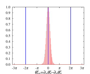
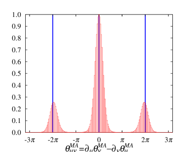
Figure 3: Histograms of $\theta_{\mu\nu}$ in Landau (Left) and MA (Right) gauges

Hence the Abelian fields satisfy kinematically the simple Abelian Bianchi identity:

$$\vec{\nabla}\times\vec{E}_{A}^{a}=\partial_{4}\vec{B}_{A}^{a},\hskip 28.45274pt\vec{\nabla}\cdot\vec{B}_{A}^{a}=0.$$ (4)

In the case of MA gauge, there are additional monopole current $(\vec{k},k_{4})$ contributions:

$$\vec{\nabla}\times\vec{E}^{MA}=\partial_{4}\vec{B}^{MA}+\vec{k},\hskip 28.45274pt\vec{\nabla}\cdot\vec{B}^{MA}=k_{4}.$$ (5)

Here $\vec{E}^{MA}$ and $\vec{B}^{MA}$ are defined in terms of plaquette variables $\theta_{\mu\nu}^{MA}(s)\ \ (\textrm{mod}\ \ 2\pi)$ which are constructed by $\theta^{MA}_{\mu}(s)$.

The Coulombic electric field coming from the static source is written in the lowest perturbation theory in terms of the gradient of a scalar potential. Hence it does not contribute to the curl of the Abelian electric field nor to the Abelian magnetic field in the above Abelian Bianchi identity Eq.(4). The dual Meissner effect says that the squeezing of the electric flux occurs due to cancellation of the Coulombic electric fields and those from solenoidal magnetic currents. In the case of MA gauge, magnetic monopole currents $\vec{k}$ play the role of the solenoidal currentSingh:1993jj ; bali-96 ; Koma:2003gq .

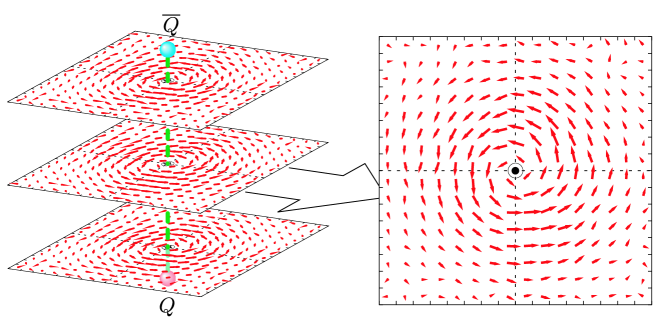
Figure 4: Magnetic displacement currents in Landau gauge as a solenoidal current.

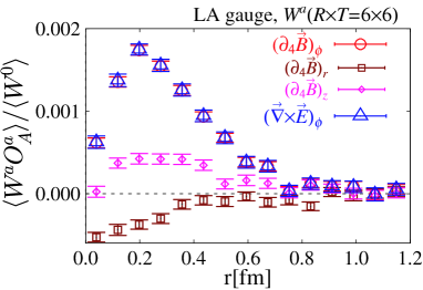
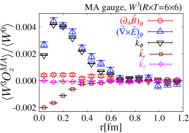
Figure 5: Curl of Abelian electric fields and magnetic displacement currents around a static quark pair in Landau (Left) and in MA (Right) gauges. Monopole currents are also plotted in MA gauge.

Now what happens in a smooth gauge like the Landau gauge where monopoles do not exist? From Eq.(4), only $\partial_{4}\vec{B}_{A}$ regarded as a magnetic displacement current could play the role of the solenoidal current. It is very interesting to see Fig.4 in which this happens actually in Landau gauge. Note that the solenoidal current has a direction squeezing the Coulombic electric field. Let us see also the detailed distributions shown in Fig.5. The other components of the magnetic displacement current $\partial_{4}B_{Ar}$ and $\partial_{4}B_{Az}$ are not vanishing but they are much suppressed consistently with Fig.2. In comparison, we show the case of MA gauge also in Fig.5. Here $\partial_{4}B_{A\phi}$ is found to be negligible numerically as already expected from the worksSingh:1993jj ; Cea:1995zt ; bali-96 . Instead monopole currents are circulatingSingh:1993jj ; bali-96 ; Koma:2003gq . In this case, $k_{r}$ is non-vanishing, although it is also suppressed in comparison with $k_{\phi}$. $k_{z}$ is almost zero. The authors think that non-vanishing of the radial and $z$ components of $\partial_{4}\vec{B}$ in Landau gauge and $\vec{k}$ in MA gauge is due to lattice artifacts and also due to the smallness of the Wilson loop size adopted here. It is interesting that the shapes of $\partial_{4}B_{A\phi}$ in Landau gauge and $k_{\phi}$ in MA gauge look similar, although the strengths are different. They have a peak at almost the same distance around $0.2$[fm] and almost vanish around $0.7$[fm].

4 Abelian dominance test

The reader may wonder if the above consideration of the Abelian fields alone is enough. Some people believe that the non-perturbative confinement problem in infrared QCD could be understood in terms of Abelian quantitiesAbelianDominance ; Reviews ; kondo-04 .

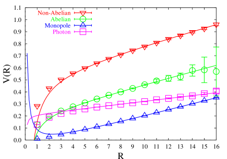
Figure 6: Abelian, monopole and photon static potentials.

First we evaluate the Abelian and monopole contributions to the string tension in MA gauge using the Iwasaki improved action (1). It is plotted in Fig.6. Our results are as follows:

$$\frac{\sigma_{ab}}{\sigma} = 0.94\pm 0.05,\ \ \ \frac{\sigma_{mo}}{\sigma_{ab}}=0.98\pm 0.02,\ \ \ \frac{\sigma_{mo}}{\sigma}=0.92\pm 0.01.$$

This is compared with the result obtained using Wilson gauge action in Ref.bali-MA :

$$\frac{\sigma_{mo}}{\sigma} = 0.87\pm 0.02$$

Hence substantial improvement is obtained with the use of Iwasaki impoved action. This suggests the abelian monopole part could reproduce the full string tension in the continuum limit.

Abelian dominance in infrared QCD is also checked in some works with the use of controlled cooling. Giedt and Greensite greensite-96 have measured the ratio $B/A$ where

$$B = -{1\over V}\sum_{x}{1\over n_{p}(n_{p}-1)}\sum_{i>j}\sum_{m>n}\mbox{Tr}\{[F_{ij}(x),F_{mn}(x)]^{2}\}$$

$$A = {1\over n_{p}V}\sum_{x}\sum_{i>j}\mbox{Tr}\{F_{ij}^{4}\}$$

and have shown that it decreases as the cooling steps as far as the string tension is kept non-vanishing. See Fig.7 taken from Ref.greensite-96 . Cooling is expected to reduce the big Coulombic interaction in the non-Abelian case while keeping infrared confinement property.

Figure 7: Non-abelianicity $Q$ vs. Cooling Step, for several values of $\beta$. This figure is from Ref.greensite-96 .

Cea and CosmaiCea:1995zt have measured connected correlation operators of Wilson loops and $1\times 1$ plaquette using the controlled cooling and have obtained the penetration length in non-Abelian case. It is almost equal to the penetration length determined by Abelian Wilson loop and Abelian electric fields in MA gauge. See Fig.8 taken from Ref.Cea:1995zt .

Figure 8: $\mu$ and $\mu_{A}$ (in units of $\Lambda_{\overline{MS}}$) versus $\beta$ for square Wilson loops. Circles, squares, and triangle refer to $L=16$, $20$, $24$ respectively. Crosses and diamond refer to the Abelian projected correlator $\rho^{A}_{W}$ with $L=16$, $20$ respectively.This figure is from Ref. Cea:1995zt .

We also try to check Abelian dominance in Landau gauge using a controlled cooling cooling under which the string tension remains non-vanishing. For reader convenience let us, briefly, illustrate our cooling procedure. The lattice gauge configurations are cooled by replacing the matrix $U_{\mu}(s)$ associated to each link $l\equiv(s,\hat{\mu})$ with a new matrix $U_{\mu}^{\prime}(s)$ in such a way that the local contribution to the lattice action

$$S(s)=1-\frac{1}{2}\text{tr}\left\{U_{\mu}(s)k(s)F(s)\right\}$$ (6)

is minimized. $\widetilde{F}(s)=k(s)F(s)$ is the sum over the “U-staples” involving the link $l$ and $k(s)=\sqrt{\text{det}\left(\widetilde{F}(s)\right)}$, so that $F(s)\in$ SU(2). In a “controlled” or “smooth” cooling step we have

$$U_{\mu}(s)\rightarrow U^{\prime}_{\mu}(s)=V(s)U_{\mu}(s)\;,$$ (7)

where $V(s)$ is the SU(2) matrix which maximizes

$$\text{tr}\left\{V(s)U_{\mu}(s)F(s)\right\}$$ (8)

subjected to the following constraint on the SU(2) distance between $U_{\mu}(s)$ and $U^{\prime}_{\mu}(s)$:

$$\frac{1}{4}\text{tr}\left[\left(U_{\mu}^{\dagger}(s)-U^{\prime\dagger}_{\mu}(s)\right)\left(U_{\mu}(s)-U^{\prime}_{\mu}(s)\right)\right]\;\leq\delta^{2}\,.$$ (9)

We adopt $\delta=0.3$. A complete cooling sweep consists in the replacement Eq. (7) at each lattice site.

We find the profile of the non-Abelian electric field $E_{z}^{a}$ tends to that of the Abelian one of $E_{Az}^{a}$ in the long-range region as shown in Fig.9. This is consistent with the above resultCea:1995zt in a different approach.

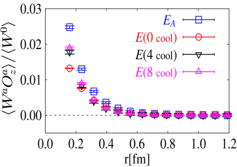
Figure 9: Profiles of non-Abelian electric field $E_{z}^{a}$ after cooling. $E_{Az}^{a}$ stands for the Abelian electric field. $W(R\times T=6\times 6)$ is used.

5 Dimension 2 gluon condensate

Now we have shown that the magnetic displacement currents are important in the dual Meissner effect when there are no monopoles. Then how can we understand the origin of the dual Meissner effect without monopoles? The Abelian dual Meissner effect indicates the massiveness of the Abelian electric field as an asymptotic field:

$$(\partial_{\rho}^{2}-m^{2})\vec{E}_{A}\sim 0.$$ (10)

This leads us to a dual London equation which is a key to the dual Meissner effect. Let us evaluate the curl of the magnetic displacement current. Using Eq.(4), we get

$$\vec{\nabla}\times\partial_{4}\vec{B}_{A} = \vec{\nabla}(\vec{\nabla}\cdot\vec{E}_{A})-\vec{\nabla}^{2}\vec{E}_{A}.$$

From Eq.(10), we get the dual London equation:

$$\vec{\nabla}\times\partial_{4}\vec{B}_{A}\sim(\partial_{4}^{2}-m^{2})\vec{E}_{A}.$$ (11)

Let us remember a simple mean-field approach developed by Fukudafukuda-82 . Neglecting gauge-fixing and Fadeev-Popov terms, we have equations of motion $D_{\mu}^{ab}F_{\mu\nu}^{b}=0$ and the (non-Abelian) Bianchi identity $D_{\mu}^{ab}{}^{*}F_{\mu\nu}^{b}=0$. Applying $D$ operator to the Bianchi identity and using the Jacobi identity and the equations of motion, we get

$$(D_{\rho}^{2})^{ab}F_{\mu\nu}^{b} = 2g\epsilon^{abc}F_{\mu\alpha}^{b}F_{\nu\alpha}^{c}.$$ (12)

Notice $(D_{\rho}^{2})^{ab}=\partial_{\rho}^{2}\delta^{ab}+g\epsilon^{acb}(\partial_{\rho}A_{\rho}^{c})+g^{2}(A_{\rho}^{a}A_{\rho}^{b}-\delta^{ab}(A_{\rho}^{c})^{2})$. Hence if $<A^{a}_{\mu}A^{b}_{\nu}>=\delta^{ab}\delta_{\mu\nu}v^{2}\neq 0$, we see asymptotically that the electric fields become massive $(\partial_{\rho}^{2}-m^{2})E^{a}_{k}\sim 0$ with $m^{2}=8g^{2}v^{2}$mass . Now the Abelian electric field is also massive asymptotically $(\partial_{\rho}^{2}-m^{2})E^{a}_{Ak}\sim 0$. Hence the dual London equation (11) is obtained.

The importance of the dimension 2 gluon condensate has been stressed by Zakharov and his collaboratorszakharov and Refs.kondo ; dudal . Recent discussions on the value of the gluon condensate are seen in Ref.arriola . Some of them discuss the mass generation of the gluon propagator. But as pointed out by Fukudafukuda-82 , the non-vanishing dimension 2 gluon condensate leads us to a conclusion that field strengths $F_{\mu\nu}^{a}(s)$ instead of gluon fields $A_{\mu}^{a}(s)$ become good canonical variables having a finite mass, whereas gluon propagators have a $(p^{2})^{-2}$ behavior showing confinement.

Although the operator of the gluon condensate is gauge-variant, it is proved recently the expectation value is gauge invariantslavnov . Hence the gluon condensate has a physical importance, if the proof is correct.

References

- (1) G. ’t Hooft, in Proceedings of the EPS International Conference, edited by A. Zichichi, p. 1225 (1976).
- (2) S. Mandelstam, Phys. Rept. 23C, 245 (1976).
- (3) G. ’t Hooft, Nucl. Phys. B190, 455 (1981).
- (4) T. Suzuki, Prog. Theor. Phys. 69, 1827(1983).
- (5) A. S. Kronfeld, M. L. Laursen, G. Schierholz and U. J. Wiese, Phys. Lett. B 198, 516 (1987); A. S. Kronfeld, G. Schierholz and U. J. Wiese, Nucl. Phys. B 293, 461 (1987).
- (6) T. Suzuki and I. Yotsuyanagi, Phys. Rev. D42, R4257 (1990);
- (7) T. Suzuki, Nucl. Phys. Proc. Suppl. 30, 176 (1993); M. N. Chernodub and M. I. Polikarpov, in ”Confinement, duality, and nonperturbative aspects of QCD”, Ed. by P. van Baal, Plenum Press, p. 387 (1997).
- (8) Y. Koma, M. Koma, E.-M. Ilgenfritz, T. Suzuki, and M. I. Polikarpov, Phys. Rev. D68, 094018 (2003).
- (9) M.N. Chernodub, Phys.Rev. D69, 094504 (2004).
- (10) J. Giedt and J. Greensite, Phys. Rev. D55, 4484 (1997).
- (11) P. Cea and L. Cosmai, Phys. Rev. D52, 5152 (1995).
- (12) The dual London equation was discussed gauge-invariantly with a definition of a non-abelian monopole current in P. Skala, M. Faber and M. Zach, Nucl. Phys. B494, 293 (1997); Phys. Lett. B424, 335 (1998).
- (13) L. Stodolsky, Pierre van Baal and V.I. Zakharov, Phys. Lett. B552, 214 (2003) and references therein.
- (14) K-I. Kondo, Phys. Lett. B514, 335 (2001); Phys.Lett. B572, 210 (2003).
- (15) D. Dudal et al., JHEP 0401, 044 (2004) and references therein.
- (16) E.R. Arriola, P.O. Bowman and W. Bronioski, ”Landau-gauge condensate from the quark propagator on the lattice”, hep-ph/0408309 and references therein.
- (17) A. A. Slavnov, ” Gauge invariance of dimension two condensate in Yang-Mills theory”, hep-th/0407194
- (18) Y.Iwasaki, Nucl. Phys. B258, 141 (1985); Univ. Tsukuba Preprint UTHEP-118(1983) unpublished.
- (19) APE Collaboration: M. Albanese et al., Phys. Lett. B192 163 (1987).
- (20) G. S. Bali, V. Bornyakov, M. Muller-Preussker and K. Schilling, Phys. Rev. D54, 2863 (1996).
- (21) G.S. Bali, K.Schilling and Ch. Schlichter, Phys. Rev. D51, 5165 (1995).
- (22) T. A. DeGrand and D. Toussaint, Phys. Rev. D22, 2478 (1980).
- (23) V. Singh D. A. Browne, and R. W. Haymaker, Phys. Lett. B306, 115 (1993).
- (24) K-I. Kondo, ”Magnetic condensation, Abelian dominance, and instability of Savvidy vacuum”, hep-th/0404252 and references therein.
- (25) G.S. Bali, V. Bornyakov, M. Mueller Preussker and K. Schilling, Phys.Rev. D54, 2863 (1996).
- (26) M.Campostrini et al., Phys. Lett. B225, 403 (1989).
- (27) R. Fukuda, Prog. Theor. Phys. 67, 648 (1982); ibid. 655 (1982).
- (28) A mass counter term is needed rigorously.