Hadron Spectrum and Decay Constant from $N_{F}=2$ Domain Wall QCD

Taku Izubuchi , [RBC Collaboration] We thank RIKEN, Brookhaven National Laboratory and the U.S. Department of Energy for providing the facilities essential for the completion of this work. This work is supported by RIKEN Super Combined Cluster at RIKEN. RIKEN-BNL Research Center, Brookhaven National Laboratory, Upton, New York 11973, USA Institute for Theoretical Physics, Kanazawa University, Kanazawa 920-1192, Japan
Abstract

We report on the first large-scale study of two flavor QCD with domain wall fermions (DWF). Simulation has been carried out at three dynamical quark mass values about 1/2, 3/4, and 1 ms​t​r​a​n​g​esubscriptπ‘šπ‘ π‘‘π‘Ÿπ‘Žπ‘›π‘”π‘’m_{strange} on $16^{3}\times 32$ volume with $L_{s}=12$ and $a^{-1}\approx 1.7$ GeV. After discussing the details of the simulation, we report on the light hadron spectrum and decay constants.

1 Introduction

We have continued to investigate two flavor QCD using dynamical DWF. We present results of the hadron spectrum and the decay constants as a project of the RBC collaboration. For other quantities on the same dynamical ensembles, see other RBC contributions in these proceedings.

In this work we choose the DBW2 gauge action at $\beta=0.80$, in which the negative coefficient to the rectangular plaquette suppresses dislocations of configuration and drastically reduces the residual mass, mr​e​ssubscriptπ‘šπ‘Ÿπ‘’π‘ m_{res}, for relatively small $L_{s}\sim O(10)$ in quenched simulation[1]. We simulated three sea quark mass ms​e​a=0.02,0.03subscriptπ‘šπ‘ π‘’π‘Ž0.020.03m_{sea}=0.02,0.03, and 0.04 using $N_{F}=2$ domain wall fermion with fifth dimensional extent $L_{s}=12$ and domain wall height $M_{5}=1.8$. $L_{s}=12$

2 Ensemble generation

Table 1: The details of $L_{s}=12,M_{5}=1.8$ DWF HMC-$\Phi$ evolution on $16^{3}\times 32$ lattice with $\beta=0.80$ DBW2 action.
$m_{\rm sea}$ $\Delta t$ Steps/Traj. Traj. $P_{acc}$ $C_{\Delta H}$ $N^{(0)}_{CG}$ $N^{(7)}_{CG}$ $N^{tot}_{CG}$ $\tau_{int}$
$0.02$ $1/100$ 51 5361 77% 16.2(2) 715 277 16014 2.9(8)
$0.03$ $1/100$ 51 6195 78% 15.8(1) 514 158 9214 3.3(5)
$0.04$ $1/80$ 41 5605 68% 16.4(2) 402 121 5964 4.5(10)

TableΒ 1 summarizes the HMC-ΦΦ\Phi evolution. An interesting result is that the acceptance, Pa​c​csubscriptπ‘ƒπ‘Žπ‘π‘P_{acc}, is insensitive to ms​e​asubscriptπ‘šπ‘ π‘’π‘Žm_{sea}. More precisely, at least for our particular run parameters: ms​e​a ∼>ms​t​r​a​n​g​e/2 ∼>subscriptπ‘šπ‘ π‘’π‘Žsubscriptπ‘šπ‘ π‘‘π‘Ÿπ‘Žπ‘›π‘”π‘’2m_{sea}\mathrel{\hbox to0.0pt{\lower 4.0pt\hbox{\hskip 1.0pt$\sim$}\hss}\raise 1.0pt\hbox{$>$}}m_{strange}/2, the squared energy difference between the first and the last configuration in a trajectory, scaled by V𝑉V and the MD step size, Δ​tΔ𝑑\Delta t,

$$C_{\Delta H}=\sqrt{\left\langle(\Delta H)^{2}\right\rangle\over V(\Delta t)^{4}}~{}~{},$$ (1)

stays same for all sea quark masses in the simulation, while an empirical estimation for staggered or Wilson fermions would be CΔ​H∼ms​e​aβˆ’Ξ±,α∼2formulae-sequencesimilar-tosubscript𝐢Δ𝐻superscriptsubscriptπ‘šπ‘ π‘’π‘Žπ›Όsimilar-to𝛼2C_{\Delta H}\sim m_{sea}^{-\alpha},\alpha\sim 2, in which case number of steps has to be increased proportional to ms​e​aβˆ’1superscriptsubscriptπ‘šπ‘ π‘’π‘Ž1m_{sea}^{-1} to keep the acceptance $P_{acc}\approx{\rm erfc}(\sqrt{\left\langle(\Delta H)^{2}\right\rangle/8})$ constant. By introducing the new force term described in [2], $C_{\Delta H}$ is reduced to $\sim$ 40 % of the old one.

We have implemented the chronological inverter technique ofΒ [3], in which the starting vector of the conjugate gradient algorithm (CG) in a MD step is forecasted by the solutions in the previous steps. $N^{(0)}_{CG}$ in the table is the number of matrix multiplication in CG without forecasting, while $N^{(7)}_{CG}$ is the count using the previous seven solutions. The number seven is about the point where the precision of the forecast is saturated. $N^{({tot})}_{CG}$ is the total number of CG count in a trajectory. By a scaling ansatz, NC​G(i)=Ci​(ms​e​a+mr​e​s)βˆ’Ξ²isubscriptsuperscript𝑁𝑖𝐢𝐺subscript𝐢𝑖superscriptsubscriptπ‘šπ‘ π‘’π‘Žsubscriptπ‘šπ‘Ÿπ‘’π‘ subscript𝛽𝑖N^{(i)}_{CG}=C_{i}(m_{sea}+m_{res})^{-\beta_{i}}, $\beta_{0}\sim 1$ and $\beta_{7}\sim 1.5$ from the table. Although $\beta_{7}>\beta_{0}$, the coefficient, $C_{i}$, is much smaller for forecasting and thus $N^{(tot)}_{CG}$ is reduced roughly by factors of two to three in the simulation points compared to the case without the forecast.

$\tau_{int}$ in the table is an estimation for the integrated auto-correlation length for $1\times 1$ plaquette using whole trajectories by the truncated sum at 50 with an error from jackknife blocks of length 100. $\tau_{int}$ are all equal within the quoted errors. The autocorrelation length of axial current correlator measured every ten trajectory is  $\mathrel{\hbox to0.0pt{\lower 4.0pt\hbox{\hskip 1.0pt$\sim$}\hss}\raise 1.0pt\hbox{$<$}}50$ trajectories111 The topological charge and the chiral condensation (with many random hits) show longer autocorrelation times.

Although these observations are encouraging for DWF simulations with lighter quark masses in the future, we note that they may only be true for relatively heavy ms​e​asubscriptπ‘šπ‘ π‘’π‘Žm_{sea}.

3 Physical Results

For each of three ms​e​asubscriptπ‘šπ‘ π‘’π‘Žm_{sea}, we measure on 94 lattices separated by 50 trajectories, leaving out the first $\simeq$ 600 trajectories to allow the evolution to thermalized. All quoted errors are from jackknife estimate of the statistical error, correlated fit to hadron propagators is made using a single covariance matrix computed on the entire ensemble.

By a linear diagonal extrapolation, ms​e​a=mv​a​lβ†’0subscriptπ‘šπ‘ π‘’π‘Žsubscriptπ‘šπ‘£π‘Žπ‘™β†’0m_{sea}=m_{val}\to 0, we found mr​e​s=0.00137​(4)subscriptπ‘šπ‘Ÿπ‘’π‘ 0.001374m_{res}=0.00137(4) or  $\mathrel{\hbox to0.0pt{\lower 4.0pt\hbox{\hskip 1.0pt$\sim$}\hss}\raise 1.0pt\hbox{$<$}}$ 5 MeV, which is larger than quenched DBW2 values for the same $L_{s}$ and $a^{-1}$, but it is still an order of magnitude smaller than the input quark mass. The impacts of mr​e​ssubscriptπ‘šπ‘Ÿπ‘’π‘ m_{res} on the operator mixing for $B_{K}$ is discussed elsewhere[4, 5].

From non-gauge-fixed wall-point pseudo-scalar correlator, $\left\langle J^{a}_{5}J^{a}_{5}\right\rangle$ we extract pseudo-scalar decay constant:

fp​s=2mp​s2​(mf+mr​e​s)β€‹βŸ¨0|J5a|Ο€,pβ†’=0⟩,subscript𝑓𝑝𝑠2superscriptsubscriptπ‘šπ‘π‘ 2subscriptπ‘šπ‘“subscriptπ‘šπ‘Ÿπ‘’π‘ quantum-operator-product0subscriptsuperscriptπ½π‘Ž5πœ‹β†’π‘0f_{ps}={2\over m_{ps}^{2}}(m_{f}+m_{res})\left\langle 0|J^{a}_{5}|\pi,\vec{p}=0\right\rangle~{}~{}, (2)

and linearly extrapolate to the chiral limit, mv​a​lq=ms​e​aq=0subscriptsuperscriptπ‘šπ‘žπ‘£π‘Žπ‘™subscriptsuperscriptπ‘šπ‘žπ‘ π‘’π‘Ž0m^{q}_{val}=m^{q}_{sea}=0 with mv​a​lq≑ms​e​a+mr​e​s,ms​e​aq=mv​a​l+mr​e​sformulae-sequencesubscriptsuperscriptπ‘šπ‘žπ‘£π‘Žπ‘™subscriptπ‘šπ‘ π‘’π‘Žsubscriptπ‘šπ‘Ÿπ‘’π‘ subscriptsuperscriptπ‘šπ‘žπ‘ π‘’π‘Žsubscriptπ‘šπ‘£π‘Žπ‘™subscriptπ‘šπ‘Ÿπ‘’π‘ m^{q}_{val}\equiv m_{sea}+m_{res},~{}m^{q}_{sea}=m_{val}+m_{res}, to obtain an estimation for its chiral value, $f=0.078(1)$. The fit to the next-to-leading order (NLO) partially quenched chiral perturbation theory (PQChPT) formula[6, 7] for $f_{ps}$ did not describe the data in the neighborhood of the fit range too well[5]. However, the following results depend on the value of $f$ only mildly, so we will use the estimation from the linear fit.

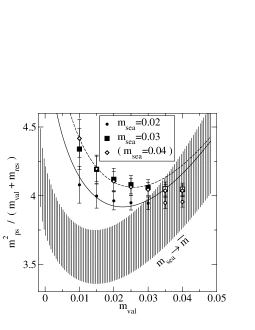
Fitting Coulomb gauge-fixed wall-point correlators, we obtain the mass of the pseudo-scalar mesons and the vector mesons. It is worth mentioning that a simple linear extrapolation of mp​s2superscriptsubscriptπ‘šπ‘π‘ 2m_{ps}^{2} to mv​a​l,s​e​aq=0subscriptsuperscriptπ‘šπ‘žπ‘£π‘Žπ‘™π‘ π‘’π‘Ž0m^{q}_{val,sea}=0 is zero within the statistical error. This did not happen in the quenched case: mp​s2=0superscriptsubscriptπ‘šπ‘π‘ 20m_{ps}^{2}=0 at mfβ‰ˆβˆ’(2βˆ’3)Γ—mr​e​ssubscriptπ‘šπ‘“23subscriptπ‘šπ‘Ÿπ‘’π‘ m_{f}\approx-(2-3)\times m_{res}[1]. This is consistent with the difference between chiral logarithms (mp​s2/mq∼2​B0+c​mq​log⁑mqsimilar-tosuperscriptsubscriptπ‘šπ‘π‘ 2superscriptπ‘šπ‘ž2subscript𝐡0𝑐superscriptπ‘šπ‘žsuperscriptπ‘šπ‘žm_{ps}^{2}/m^{q}\sim 2B_{0}+cm^{q}\log m^{q}) vs the quenched one (mp​s2/mq∼log⁑mqsimilar-tosuperscriptsubscriptπ‘šπ‘π‘ 2superscriptπ‘šπ‘žsuperscriptπ‘šπ‘žm_{ps}^{2}/m^{q}\sim\log m^{q}) at small $m^{q}$.

The NLO PQChPT formula,

$\displaystyle M^{2}_{\pi,K(1-loop)}=M^{2}\left(1+\frac{\Delta M^{2}}{M^{2}}\right)$ (3)
$\displaystyle\frac{\Delta M^{2}}{M^{2}}=\frac{2}{N}\!\!\left[\frac{M^{2}\!-\!M^{2}_{SS}}{16\pi^{2}f^{2}}+\frac{2M^{2}-M^{2}_{SS}}{M^{2}}A_{0}(M^{2})\right]$
$\displaystyle\ \ \ -\frac{16}{f^{2}}[(L_{5}-2L_{8})M^{2}+(L_{4}-2L_{6})NM^{2}_{SS}],$ (4)

with

$\displaystyle M^{2}$ $\displaystyle=$ 2​B0​mv​a​lq,MS​S2=2​B0​ms​e​aq,2subscript𝐡0subscriptsuperscriptπ‘šπ‘žπ‘£π‘Žπ‘™subscriptsuperscript𝑀2𝑆𝑆2subscript𝐡0subscriptsuperscriptπ‘šπ‘žπ‘ π‘’π‘Ž\displaystyle{2\,B_{0}}\,m^{q}_{val}~{},~{}M^{2}_{SS}={2\,B_{0}}\,m^{q}_{sea}~{}, (5)
$\displaystyle A_{0}(M^{2})$ $\displaystyle=$ $\displaystyle\frac{1}{16\pi^{2}f^{2}}M^{2}\ln\frac{M^{2}}{\Lambda_{\chi}^{2}}~{}~{},$ (6)

is used to fit the pseudo-scalar mass obtained from axial current correlators and pseudo-scalar correlators for various mass ranges. The NLO fit is constrained as mp​s2=0superscriptsubscriptπ‘šπ‘π‘ 20m_{ps}^{2}=0 at mv​a​l=βˆ’mr​e​ssubscriptπ‘šπ‘£π‘Žπ‘™subscriptπ‘šπ‘Ÿπ‘’π‘ m_{val}=-m_{res}, as it must due to the universality of the low energy domain wall fermion theory, and $f$ estimated above is used as an input. The results of fit of the fit are shown in FigureΒ 1 and in TableΒ 2. Note that $B_{0}$ is stable under change of fitting range, while the $L_{i}$ coefficients are not. When the heavier mass is included in the fit, the $\chi^{2}/dof$ increases.

Table 2: Parameters from chiral perturbation theory fits to the values of mp​s2superscriptsubscriptπ‘šπ‘π‘ 2m_{ps}^{2} at mf=ms​e​a,v​a​l≀mf(m​a​x)subscriptπ‘šπ‘“subscriptπ‘šπ‘ π‘’π‘Žπ‘£π‘Žπ‘™superscriptsubscriptπ‘šπ‘“π‘šπ‘Žπ‘₯m_{f}=m_{sea,val}\leq m_{f}^{(max)} computed from the pseudo-scalar wall-point (upper two column), and axial-vector wall point. $\chi^{2}$ is from uncorrelated fits in $m_{f}$. $L_{i}$ refer to Gasser-Leutwyler low energy constants multiplied by $10^{4}$ at $\Lambda_{\chi}=1$ GeV.
$m_{f}^{(max)}$ $\chi^{2}/$dof $2\,B_{0}$ $L_{5}-2L_{8}$ $L_{4}-2L_{6}$
0.03 $0.1(1)$ $4.0(3)$ $-1.5(7)$ $-2(1)$
0.04 $2(1)$ $4.2(1)$ $-0.2(4)$ $-1.1(4)$
0.03 $0.3(2)$ $4.0(3)$ $-1.9(8)$ $-1(1)$
0.04 $1.9(9)$ $4.2(1)$ $-0.4(4)$ $-0.8(3)$
Refer to caption
Figure 1: mp​s2/(mv​a​l+mr​e​s)subscriptsuperscriptπ‘š2𝑝𝑠subscriptπ‘šπ‘£π‘Žπ‘™subscriptπ‘šπ‘Ÿπ‘’π‘ m^{2}_{ps}/(m_{val}+m_{res}) as a function of $m_{val}$ for each ms​e​a=0.04,0.03,0.02subscriptπ‘šπ‘ π‘’π‘Ž0.040.030.02m_{sea}=0.04,0.03,0.02. The curves are from the results of NLO fit using ms​e​a,v​a​l≀0.03subscriptπ‘šπ‘ π‘’π‘Žπ‘£π‘Žπ‘™0.03m_{sea,val}\leq 0.03.

A linear extrapolation of the three vector meson mass points mv​a​l=ms​e​asubscriptπ‘šπ‘£π‘Žπ‘™subscriptπ‘šπ‘ π‘’π‘Žm_{val}=m_{sea}, yields $a^{-1}=$1.69(5) GeV at the quark mass, $m_{f}=\bar{m}=0.0002(1)$ corresponding to the neutral pion mass using (3). Similarly, but using the NLO ChPT prediction for non-degenerate valence quarks, ms=0.045​(3)subscriptπ‘šπ‘ 0.0453m_{s}=0.045(3) is obtained from the physical kaon mass. The coefficients in the NLO formula for non-degenerate quarks are determined by the fit of the degenerate quark meson. It is important to note that $\bar{m}$ and mssubscriptπ‘šπ‘ m_{s} as defined above are bare quark masses; the renormalized quark mass is defined as Zm​mq=Zm​(m+mr​e​s)subscriptπ‘π‘šsuperscriptπ‘šπ‘žsubscriptπ‘π‘šπ‘šsubscriptπ‘šπ‘Ÿπ‘’π‘ Z_{m}m^{q}=Z_{m}(m+m_{res}), where $Z_{m}$ is a scheme and scale dependent renormalization factor[2].

Extrapolating the measured decay constant at the partially quenched points (mv​a​l,s​e​a≀0.04subscriptπ‘šπ‘£π‘Žπ‘™π‘ π‘’π‘Ž0.04m_{val,sea}\leq 0.04) using the linear ansatz to $\bar{m}$ and mssubscriptπ‘šπ‘ m_{s}, we find $f_{\pi}=134(4)$ MeV, $f_{K}=157$(4) MeV, and $f_{K}/f_{\pi}=1.18(1)$, which agree better with experiment than quenched DWF simulations.

Sommer scale, $r_{0}$ (with $r_{0}=0.5$fm ), from the static quark potential gives almost the same value for the lattice spacing [8]. A similar analysis has been carried out for baryons, and the chiral limit of the linear extrapolation gives $M_{N}/M_{\rho}$ = 1.34(4), which is larger than the experimental value. This would be expected from the relatively small spatial volume.

4 Conclusion

We have generated configurations of lattice QCD with two-flavor dynamical DWF at aβˆ’1β‰ˆ1.7superscriptπ‘Ž11.7a^{-1}\approx 1.7 GeV, with a spacial volume Vβ‰ˆ(1.9​fm)3𝑉superscript1.9fm3V\approx(1.9{\rm fm})^{3}. From the ∼3Γ—5000similar-toabsent35000\sim 3\times 5000 trajectories in this work obtained with light dynamical quarks and small residual quark mass, ms​t​r​a​n​g​e/2<∼ms​e​a+mr​e​s<∼ms​t​r​a​n​g​e<∼subscriptπ‘šπ‘ π‘‘π‘Ÿπ‘Žπ‘›π‘”π‘’2subscriptπ‘šπ‘ π‘’π‘Žsubscriptπ‘šπ‘Ÿπ‘’π‘ <∼subscriptπ‘šπ‘ π‘‘π‘Ÿπ‘Žπ‘›π‘”π‘’m_{strange}/2\mathrel{\hbox to0.0pt{\raise 2.20013pt\hbox{$<$}\hss}{\lower 2.20013pt\hbox{$\sim$}}}m_{sea}+m_{res}\mathrel{\hbox to0.0pt{\raise 2.20013pt\hbox{$<$}\hss}{\lower 2.20013pt\hbox{$\sim$}}}m_{strange} or 0.54<∼mp​s/mV<∼0.65<∼0.54subscriptπ‘šπ‘π‘ subscriptπ‘šπ‘‰<∼0.650.54\mathrel{\hbox to0.0pt{\raise 2.20013pt\hbox{$<$}\hss}{\lower 2.20013pt\hbox{$\sim$}}}m_{ps}/m_{V}\mathrel{\hbox to0.0pt{\raise 2.20013pt\hbox{$<$}\hss}{\lower 2.20013pt\hbox{$\sim$}}}0.65. We have tried the NLO ChPT fit for the mass and a simple linear fit for the decay constant. The results for the physical decay constants are closer than those in quenched DWF simulation. For further details of the simulations and results, we refer the reader to the forthcoming paper[5].

References

  • [1] Y. Aoki etΒ al., Phys. Rev. D69 (2004) 074504, hep-lat/0211023.
  • [2] RBC, C. Dawson, Nucl. Phys. Proc. Suppl. 128 (2004) 54, hep-lat/0310055.
  • [3] R.C. Brower etΒ al., Nucl. Phys. B484 (1997) 353, hep-lat/9509012.
  • [4] RBC, C. Dawson, in these proceedings.
  • [5] RBC, Y. Aoki etΒ al., forthcoming.
  • [6] M.F.L. Golterman and K.C. Leung, Phys. Rev. D57 (1998) 5703, hep-lat/9711033.
  • [7] J. Laiho and A. Soni, Phys. Rev. D65 (2002) 114020, hep-ph/0203106.
  • [8] RBC, K. Hashimoto and T. Izubuchi, in these proceedings.