Kaon matrix elements in domain-wall QCD with DBW2 gauge action

Abstract

We present calculations of the decay constants and kaon B-parameter $B_{K}$ as the first stage of RBC Collaboration’s quenched numerical simulations using DBW2 gauge action and domain-wall fermions. Some of potential systematic errors and consistency to previous works are discussed.

1 Introduction

In the quantities related to kaon physics such as $f_{\pi}$, $f_{K}$, $B_{K}$, ${\rm Re}A_{0}/{\rm Re}A_{2}$ and $\epsilon^{\prime}/\epsilon$, the first three are constructed straightforwardly on the lattice. However, in actual numerical simulations, there are several potential sources of systematic error, namely explicit breaking of chiral symmetry, scaling violation, finite volume effect and quenching effect. Although many efforts have been made to decrease these errors, yet more numerical simulations should be done to attain a conclusion.

We report our results of $f_{\pi}$, $f_{K}$ and $B_{K}$ as a conclusion of the first stage of our longstanding quenched numerical simulations using domain-wall fermion and DBW2 gauge action. By our choice of the lattice action, it is expected that the contamination from the explicit chiral symmetry breaking is vanishingly small. In particular, we estimate the effect of operator mixing in the calculation of $B_{K}$ through the non-perturbative calculation of the renormalization factors which weight contributions of the mixing operators. We also examine the scale dependence of our results by carrying out two kinds of numerical simulations with a similar physical lattice volume $\approx 1.6$ fm but with different scales $a^{-1}\approx$ 2 GeV and 3 GeV. After comparing our results with those from previous works, we present our continuum results of $B_{K}$.

For other kind of RBC’s numerical simulations with the dynamical quark, see ref. [1].

2 Numerical Simulations

Table 1: Simulation parameters, statistics and results of $a^{-1}$, $m_{\rm res}a$, $Z_{A}$ and $m_{s}a/2$.

$\beta$	$1.22$	$1.04$
size	$24^{3}\times 48$	$16^{3}\times 32$
$M_{5}a$	$1.65$	$1.8$
$L_{s}$	$10$	$16$
$m_{f}a$	0.008 – 0.040	0.01 – 0.05
	in step of 0.008	in steps of 0.01
#configs.
($Z_{B_{K}}$)	53	50
(others)	106	202
basic results
$a^{-1}$	2.914(54) GeV	1.982(21) GeV
$m_{\rm res}a$	$9.73(4)\cdot 10^{-5}$	$1.85(12)\cdot 10^{-5}$
$Z_{A}$	0.88813(19)	0.84019(17)

In Table 1, we enumerate two sets of our simulation parameters, statistics and results of the basic quantities such as lattice scale from the input $m_{\rho}=770$ MeV, the residual quark mass $m_{\rm res}$ and the renormalization factor of axial vector $Z_{A}$. Results of the basic quantities for $\beta=1.04$ are quoted from ref. [2], in particular. For the finer lattice with $\beta=1.22$, it is known that the topological charge $Q_{\rm top}$ changes very slowly in the ordinary Markov chain [2]. To avoid incorrect distribution of $Q_{\rm top}$, we generated configurations as described in ref. [3]. As a result, we obtained a reasonable distribution of the topological charge: $\left\langle Q_{\rm top}\right\rangle=0.38(29)$. We employ the averaged quark propagator over those with periodic and anti-periodic boundary conditions in the temporal direction for the calculation of $f_{\pi}$, $f_{K}$ and $B_{K}$. Therefore, temporal lattice size may be treated as 96 and 48 for $\beta=1.22$ and $1.04$.

3 Decay Constants

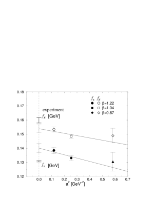
Figure 1: Results of $f_{\pi}$ (filled symbols) and $f_{K}$ [GeV] (open symbols) versus $a^{2}\ [{\rm GeV}^{-2}]$.

As a combination of fit parameters of two point correlation functions of mesons, we calculate decay constants of the pseudo-scalar from the combination of the fit parameters:

$$f_{PS}=\frac{{\cal A}^{A_{4}P}_{\rm pw}}{\sqrt{\frac{m_{\rm PS}}{2}V{\cal A}^{PP}_{\rm ww}}},$$ (1)

where ${\cal A}^{A_{4}P}_{\rm pw}$ and ${\cal A}^{PP}_{\rm ww}$ are the amplitudes of the correlation functions $\left\langle A^{\rm point}_{4}(t)P^{\rm wall}(0)\right\rangle$ and $\left\langle P^{\rm wall}(t)P^{\rm wall}(0)\right\rangle$. $m_{PS}$ is determined from the simultaneous fit of these two correlation functions thus common to both. Using the linear fit with $f_{PS}=c_{0}+c_{1}m_{PS}^{2}$, we extract bare values of $f_{\pi}$ at $m_{PS}=m_{\pi}$ and $f_{K}$ at $m_{PS}=m_{K}$. Multiplying these values by $Z_{A}$ in Table 1, we show our physical results in Figure 1. As well as for $\beta=1.22$ (circles) and $1.04$ (squares), results for $\beta=0.87$ (diamonds) from ref. [2] are plotted in this figure. By the linear fit using these three data, our results are $f_{\pi}=$ 140.1(3.3) MeV and $f_{K}=$153.9(2.6) MeV in the continuum limit. They are both inconsistent with the experimental values. On the other hand, our result $f_{K}/f_{\pi}=1.098(13)$ in the continuum limit is roughly consistent with the estimation from the quenched chiral perturbation theory [4].

4 Kaon B-parameter $B_{K}$

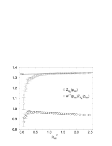
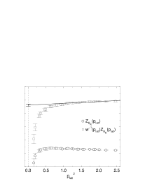
Figure 2: $Z_{B_{K}}$ and RGI value $\hat{Z}_{B_{K}}$ versus $p_{\rm latt}^{2}$ for DBW2 $\beta=1.22$ (left) and $\beta=1.04$ (right). In each panel, $Z_{B_{K}}$ (circles), RGI value (squares) and its linear extrapolation are shown.

We compute $B_{PS}$ i.e. $B_{K}$ on the lattice, by extracting a plateau of the ratio of the correlation functions:

$$\frac{\left\langle 0\left|P^{\rm wall}(t^{\prime}_{0})Q_{\Delta S=2}(t)P^{\rm wall}(t_{0})\right|0\right\rangle}{\frac{8}{3}\left\langle 0\left|P^{\rm wall}(t^{\prime}_{0})A_{4}(t)\right|0\right\rangle\left\langle 0\left|A_{4}(t)P^{\rm wall}(t_{0})\right|0\right\rangle},$$ (2)

where the locations of two wall sources $P^{\rm wall}$ are $(t_{0},t^{\prime}_{0})=(7,41)$ and $(5,27)$ for $\beta=1.22$ and $1.04$. We chose $19\leq t\leq 29$ and $14\leq t\leq 17$ for the fit ranges in each case.

To determine the renromalization factor $Z_{B_{K}}$, we employ the non-perturbative calculation which was pioneered by ref. [5]. Including the possibility of the contribution from the mixing operators, the renormalization condition is written by

$$Z_{q}^{-2}Z_{ij}\Gamma^{(4){\rm latt}}_{{\cal O}_{j}}(p_{\rm latt})=\Gamma^{(4){\rm tree}}_{{\cal O}_{i}},$$ (3)

where $\Gamma^{(4){\rm latt}}_{{\cal O}_{j}}$ and $\Gamma^{(4){\rm tree}}_{{\cal O}_{j}}$ are the amputated four point vertices on the lattice and in the tree level for the four-quark operator ${\cal O}_{j}$ with certain chiralities $i=VV\pm AA,\ SS\mp PP$ and $TT$. By solving (3), we observe that the renormalization factors $Z_{ij}$ for the mixing operators are at most $\sim 0.1\%$ of the factor for $VV+AA$, which corresponds to $Q_{\Delta S=2}$. These small $Z_{ij}$’s suppress the effect of the operator mixing to be less than the statistical error of $B_{PS}$ in spite of the fact the B-parameters of the mixing operators are a few dozens times larger than $B_{PS}$ [6].

In Figure 2, we show the results $Z^{\rm RI/MOM}_{B_{K}}=Z_{VV+AA,VV+AA}/Z_{A}^{2}$ in RI/MOM scheme and the renormalization group independent (RGI) value $\hat{Z}_{B_{K}}=w^{-1}_{\rm RI/MOM}(p_{\rm latt})Z^{\rm RI/MOM}(p_{\rm latt})$, where the factor $w^{-1}_{\rm RI/MOM}$ was calculated in ref. [7]. Extrapolating the data for $p_{\rm latt}>1$ linearly, we quote $\hat{Z}_{B_{K}}$ at $p_{\rm latt}=0$. Renormalization factor in the $\overline{\rm MS}$, NDR scheme are calculated as $Z^{\overline{\rm MS}}_{B_{K}}=w_{\overline{\rm MS}}(\mu=2\ {\rm GeV})\hat{Z}_{B_{K}}$.

We plot renormalized value $B^{\rm(ren)}_{PS}=Z^{\overline{\rm MS}}_{B_{K}}(\mu=2\ {\rm GeV})B_{PS}$ as a function of $m_{PS}^{2}\ [{\rm GeV}^{2}]$ in Figure 3, where circles are from $\beta=1.22$ and squares from $1.04$. Using the chiral expansion [8]

$$B_{PS}=\xi_{0}\left[1-\frac{6}{(4\pi f)^{2}}m^{2}_{PS}\ln\frac{m_{PS}^{2}}{\Lambda_{\chi}^{2}}\right]+\xi_{1}m_{PS}^{2},$$ (4)

and our results of $f_{PS}(m_{PS}=0)$ for the coefficient of the chiral log, we obtain the solid and dashed curves for $\beta=1.22$ and $1.04$ with $\chi^{2}/$dof = 0.80 and 0.08, respectively. Result of $B_{K}^{\overline{\rm MS}}(\mu=2\ {\rm GeV})$ for each $\beta$ from the interpolation to $m_{PS}=m_{K}$ are shown by the filled symbols in Figure 4. In the same figure, we plot results of CP-PACS [9] using Iwasaki gauge action with two set of similar parameters as ours, i.e. $(a^{-1}=2.87\ {\rm GeV},\ 24^{3}\times 60,\ L_{s}=16)$ and $(a^{-1}=1.88\ {\rm GeV},\ 16^{3}\times 40,\ L_{s}=16)$ with the open squares. On the other hand, the open circle corresponds to the previous result of RBC [10] using Wilson gauge action with $(a^{-1}=1.922(40)\ {\rm GeV},\ 16^{3}\times 32,\ L_{s}=16)$. For $a^{-1}\approx$ 2 GeV, results from these three kinds of calculations distribute over the width of more than 10%. On the other hand, for $a^{-1}\approx 3$ GeV, results from both Collaboration agree with each other. In the continuum limit taken by the naive extrapolation of our two results, we extract $B_{K}^{\overline{\rm MS}}(\mu=2\ {\rm GeV})=0.569(21)$ and $\hat{B}_{K}=0.762(28)$.

Figure 3: $B^{\rm(ren)}_{PS}$ vs. $m_{\pi}^{2}\ [{\rm GeV}^{2}]$ with fit curves.

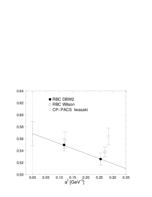
Figure 4: $B_{K}$ versus $a^{-2}\ [{\rm GeV}^{-2}]$. As well as our results (filled symbols), we quoted previous results from refs. [9, 10] (open symbols).

References

- [1] See contributions of C. Dawson, T. Izubuchi to these proceedings.
- [2] Y. Aoki et al. (RBC Collaboration), Phys. Rev. D69 (2004) 074504.
- [3] J. Noaki for RBC Collaboration, Nucl. Phys. B (Proc. Suppl.) 119 (2003) 362.
- [4] C. Bernard and M. F. L. Golterman, Phys. Rev. D46 (1992) 853.
- [5] G. Martinelli et al., Nucl. Phys. B445 (1995) 81; T. Blum et al. (RBC Collaboration), Phys. Rev. D66 (2002) 014504.
- [6] RBC Collaboration, in preparation.
- [7] M. Ciuchini et al., Nucl. Phys. B523 (1998) 501.
- [8] Sharpe, S., Phys. Rev. D46 (1992) 3146.
- [9] A. Ali Khan et al. (CP-PACS Collaboration), Phys. Rev. D64 (2001) 114506.
- [10] T. Blum et al. (RBC Collaboration), Phys. Rev. D68 (2003) 114506.