HU-EP-04/61 SFB/CPP-04-55
Universality in the Gross-Neveu model

Abstract

We consider universal finite size effects in the large-$N$ limit of the continuum Gross-Neveu model as well as in its discretized versions with Wilson and with staggered fermions. After extrapolation to zero lattice spacing the lattice results are compared to the continuum values.

1 Introduction

The treatment of fermions in lattice simulations requires special care, and several different formulations have been found over the years. Since Aoki’s lattice-2000 plenary talk [1] one may wonder, whether the models using Wilson-fermions and the staggered formulation really lie in the same universality class. It is difficult to clarify the situation in a four dimensional theory, where due to numerical costs the achievable statistical errors are too high for precision checks. Hence we decided to investigate a two dimensional toy model, which is also accessible to analytical calculations.

For our study we choose the Gross-Neveu model, defined by the Euclidean action density

$$\mathcal{L}=\bar{\psi}_{i}\not{\partial}\psi_{i}-\frac{\lambda}{2N}(\bar{\psi}_{i}\psi_{i})^{2}\,.$$ (1)

The fields $\psi_{i}$ are two component spinors and $i=1\ldots N$ is a flavor index. The action possesses an $O(2N)$ flavor symmetry [3] and is invariant under discrete chiral transformations

$$\psi_{i} \to \gamma_{5}\psi_{i}$$

$$\bar{\psi}_{i} \to -\bar{\psi}_{i}\gamma_{5}\,.$$ (2)

Spontaneous breakdown of this $\gamma_{5}$-symmetry leads to a dynamical mass generation [2]. Moreover the model is renormalizable, asymptotically free and large-$N$ expandable. The large-$N$ limit is taken keeping the dimensionless coupling constant $\lambda$ fixed.

An equivalent action, which is bilinear in the fermion fields results from the introduction of an auxiliary scalar field $\sigma$

$$\mathcal{L}^{\sigma}=\bar{\psi}_{i}(\not{\partial}+\sigma)\psi_{i}+\frac{N}{2\lambda}\sigma^{2}\,.$$ (3)

2 Large-$N$ calculation

In leading order of the large-$N$ expansion the fermion mass $m$ is given by the value of the constant field $\sigma$ that satisfies the gap-equation

$$\frac{\sigma}{\lambda}=\frac{1}{TL}{\rm tr}(\not{\partial}+\sigma)^{-1}\,,$$ (4)

where $L$ is the spatial and $T$ the temporal extent. In our notation $m(L)$ denotes the finite volume fermion-mass, and $m(\infty)\equiv m$. We are interested in the universal curve $m(L)L$ versus $mL$, similar to the Lüscher-Weisz-Wolff-coupling [4].

2.1 Continuum

In the continuum theory the calculation can be performed in analogy to the finite temperature calculation [5]. In infinite volume the gap-equation can be solved in closed form. It has solutions at $\sigma=0$ (maximum of the effective potential) as well as at $\sigma=\pm m$ (minima) with

$$m=\frac{\Lambda}{\sinh\frac{\pi}{\lambda}}\,,$$ (5)

where $\Lambda$ is a cutoff on the spatial momentum. In finite volume ($L$ finite, $T\to\infty$) we have to specify the spatial boundary conditions. Our choice are b.c. of the form $\psi(x_{0},x_{1}+L)=e^{i\theta}\psi(x_{0},x_{1})$ which include periodic and antiperiodic b.c. as special cases. Eq. (5) can be used to eliminate the bare parameter $\lambda$ in the finite volume gap-equation. The physical scale in the renormalized theory is given by $m$, which is kept constant while the cutoff is removed, allowing us to find solutions $m(L)L$ versus $mL$. Fig. 1 shows the results which strongly depend on the chosen angle $\theta$. For all $-\pi<\theta<\pi$ different from zero there is a “critical volume” below which no spontaneous symmetry breaking takes place

$$L_{c}=\frac{4\pi}{m}\exp\left[-\frac{\pi}{|\theta|}-\gamma-\sum_{n=1}^{\infty}\left(\frac{\theta}{2\pi}\right)^{2n}\zeta(2n+1)\right]\,,$$

where $\gamma$ is the Euler-Mascheroni-constant and $\zeta$ the Riemann-zeta-function.

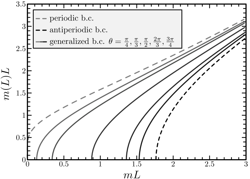
Figure 1: Universal curves $m(L)L$ versus $mL$ obtained from solutions of the gap-equation of the continuum Gross-Neveu model.

2.2 Wilson fermions

The Wilson term breaks chiral symmetry explicitly which can lead to difficulties. The Gross-Neveu model with Wilson fermions was pioneered by Aoki and Higashijima [6]. The authors found that in order to recover the $\gamma_{5}$-symmetry in the continuum limit, it is necessary to introduce a bare mass parameter $m_{0}$ and tune it to a critical value. The fermion mass $m$ can be defined as half of the distance between the two degenerate (at critical $m_{0}$) minima of the effective potential

$$V_{\rm eff}=\frac{\sigma^{2}}{2\lambda}-\frac{1}{TL}{\rm tr}\ln(D_{W}+\sigma+m_{0})\,,$$ (6)

which is not symmetric at finite lattice spacing $a$ (Fig. 2). $D_{W}$ is the free Wilson-Dirac operator. This definition of $m$ coincides with that in the continuum theory for $a\to 0$.

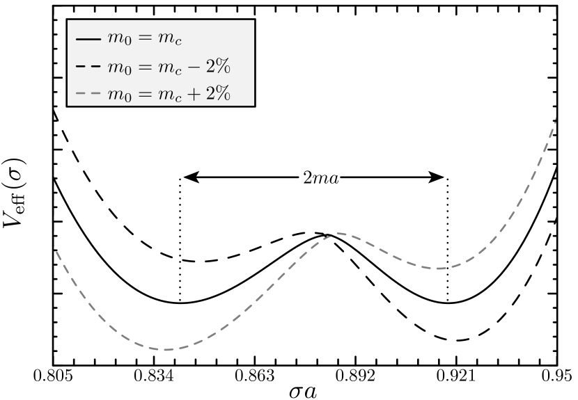
Figure 2: The effective potential with Wilson fermions for some values of $m_{0}$ around the critical one. $L/a=T/a=\infty$.

From fermion masses in finite and infinite volume we can construct curves corresponding to those in Fig. 1 for a series of lattice spacings. The approach to the continuum for a fixed value of $mL$ is shown in Fig. 3.

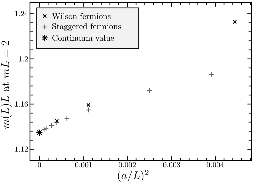
Figure 3: Approach of $m(L)L$ to the continuum value at $mL=2$ for staggered- and Wilson-fermions. Antiperiodic boundary conditions.

2.3 Staggered fermions

With Kogut-Susskind fermions it first has to be clarified how to treat the four fermion interaction. One method is to perform the spin diagonalization within the free theory, keep only one component of the fields ($\bar{\chi},\chi$) and construct taste fields ($\bar{q},q$) from one-component fields within a hypercube (a square in 2d). Once the taste fields are constructed, the four-fermion interaction $(\bar{q}q)^{2}$ can be written down and expressed in terms of the one-component fields, which leads to the action

$$S = \sum_{x}\bar{\chi}_{i}(x)\eta_{\mu}\tilde{\partial}_{\mu}\chi_{i}(x)$$

$$- \frac{\lambda}{N}\sum_{X}\left(\sum_{\rho}\bar{\chi}_{i}(2X+\rho)\chi_{i}(2X+\rho)\right)^{2}\,.$$

$X$ denotes the hypercubes and $\rho$ the position within a hypercube, such that $x=2X+\rho$. In two dimensions the phases are given by $\eta_{\mu}=(-1)^{\mu x_{0}}$. The symbol $\tilde{\partial}_{\mu}$ stands for the symmetric lattice derivative. Again the four-fermion interaction term can be traded for a scalar field. In [7] it was pointed out, that the lack of translation symmetry by one lattice spacing complicates a perturbative treatment of this model. An alternative staggered action, which cures this problem has got the interaction term

$$\frac{\lambda}{4N}\sum_{x}\left(\sum_{\rho}\bar{\chi}_{i}(x+\rho)\chi_{i}(x+\rho)\right)^{2}$$ (8)

Both formulations lead to the gap-equation

$$\frac{2\sigma}{\lambda}=\frac{1}{TL}{\rm tr}(\eta_{\mu}\tilde{\partial}_{\mu}+\sigma)^{-1}\,.$$ (9)

Numerical solutions at a fixed $mL$ for different lattice spacings are shown in Fig. 3.

3 Conclusions

Our large-$N$ calculation in the Gross-Neveu model allows for the following conclusions:

• Both the naive staggered and the Wilson formulation lead to the correct continuum limit of the finite volume massgap.

• As in QCD, with Wilson fermions an additive mass renormalization is necessary, which is absent with staggered fermions.

• With staggered fermions the construction of physical fields is more involved and special care has to be taken when interactions are introduced.

It should be mentioned however, that the leading order of the large-$N$ expansion is insensitive to problems that might occur at finite $N$. Therefore a calculation of the $1/N$-correction would be desirable. In a Monte-Carlo study at finite $N$ some additional problems will show up, e.g. the lack of true spontaneous symmetry breaking in finite volume at finite $N$ and the problem of determining the critical bare mass with Wilson fermions.

Eventually we plan also to investigate the taste reduction by taking fractional powers of the staggered determinant. There the question is open, whether a local fermion operator can be identified to give a solid basis to this approach [8].

References

- [1] S. Aoki, Nucl. Phys. Proc. Suppl. 94, 3 (2001)
- [2] D. J. Gross and A. Neveu, Phys. Rev. D 10, 3235 (1974).
- [3] R. F. Dashen, B. Hasslacher and A. Neveu, Phys. Rev. D 12, 2443 (1975).
- [4] M. Lüscher, P. Weisz and U. Wolff, Nucl. Phys. B 359, 221 (1991).
- [5] U. Wolff, Phys. Lett. B 157, 303 (1985).
- [6] S. Aoki and K. Higashijima, Prog. Theor. Phys. 76, 521 (1986).
- [7] T. Jolicoeur, A. Morel and B. Petersson, Nucl. Phys. B 274, 225 (1986).
- [8] B. Bunk, M. Della Morte, K. Jansen and F. Knechtli, Nucl. Phys. B 697, 343 (2004)