Heavy-light decay constants using clover valence quarks and three flavors of dynamical improved staggered quarks

Abstract

Starting in 2001, the MILC Collaboration began a large scale calculation of heavy-light meson decay constants using clover valence quarks on ensembles of three flavor configurations. For the coarse configurations, with $a=0.12$ fm, eight combinations of dynamical light and strange quarks have been analyzed. For the fine configurations, with $a=0.09$ fm, three combinations of quark masses are studied. Since we last reported on this calculation, statistics have been increased on the fine ensembles, and, more importantly, a preliminary value for the perturbative renormalization of the axial-vector current has become available. Thus, results for $f_{B}$, $f_{B_{s}}$, $f_{D}$ and $f_{D_{s}}$ can, in principle, be calculated in MeV, in addition to decay-constant ratios that were calculated previously.

1 INTRODUCTION

Calculation of heavy-light meson decay constants is important for the extraction of a number of CKM matrix elements. For example, $\Gamma(D^{+}_{s}\rightarrow l^{+}\nu_{l})\propto f^{2}_{D_{s}}|V_{cs}|^{2}$. As decay constants are fairly easy to determine in lattice calculations and they will be measured at BaBar, KEK and CLEO-c, they provide an excellent opportunity to verify the accuracy of our methods.

We are extending a calculation of heavy-light meson decay constants with three flavors of dynamical quarks that was begun in 2001 [1]. In this calculation, clover quarks are used for both the light and heavy valence quarks, the latter with the Fermilab interpretation [2]. A collaboration of Fermilab and MILC is now using light Asqtad quarks with the same dynamical gauge configurations to calculate decay constants. The newer calculation [3] will allow better control of chiral extrapolations, as it is practical to reduce the light valence quark mass. However, for $D_{s}$ and $B_{s}$ we expect the two approaches to be complimentary.

Since the last time we reported on this calculation [4], we have greatly increased the statistics on two gauge ensembles with $a=0.09$ fm. (See Table 1.) Furthermore, preliminary results from a one-loop perturbative calculation of the axial-vector renormalization constant $Z_{A}$ have been provided by El-Khadra, Nobes and Trottier [5].

dynamical	$\beta$	configs.	configs.
$am_{u,d}/am_{s}$		generated	analyzed
$a=0.09$ fm; $28^{3}\times 96$
0.031/0.031	7.18	496	163 (163)
0.0124/0.031	7.11	527	242 (120)
0.0062/0.031	7.09	592	293 (48)

Table 1: Details of fine lattice configurations. In parentheses are the numbers of configurations analyzed in Ref. [4].

Dynamical gauge configurations are generated using the Asqtad action [6]. Further details of confiuration generation may be found in Ref. [7]. For each ensemble of dynamical quark configurations, we use five light and five heavy valence quark masses. The masses and decay constants are interpolated or extrapolated as explained below to get physically relevant values. The relative scale is set through the heavy quark potential [7] and the overall scale is set from bottomonium splittings.

2 ANALYSIS OF RESULTS

The analysis of the heavy-light decay constants involves a number of steps. On each ensemble studied, we:

1. fit light pseudoscalar (PS) hadron propagators to determine PS masses

2. perform a quadratic chiral fit of squared PS masses to determine $\kappa_{c}$

3. determine $m_{s}$ from the mass of $\bar{s}s$ pseudoscalar state assuming a linear chiral mass relation

4. fit heavy-light (HL) channels to determine their masses and decay amplitudes

5. extrapolate or interpolate results in light quark mass to $m_{u,d}$ or $m_{s}$, respectively (see Fig. 1). We see that the interpolation required for the strange quark mass is well under control. However, in extrapolating to $m_{u,d}$, we are expected to find chiral logarithms [8]. With clover light quarks, it is a long extrapolation to the physical value of $m_{u,d}$ and it is not possible to see the chiral logs. This difficulty is much improved with Asqtad light quarks [3]. We could also consider an extrapolation of decay constant ratios, such as $f_{B}/f_{\pi}$ or $(f_{B_{s}}/f_{B})/(f_{K}/f_{\pi})$ [9].

   

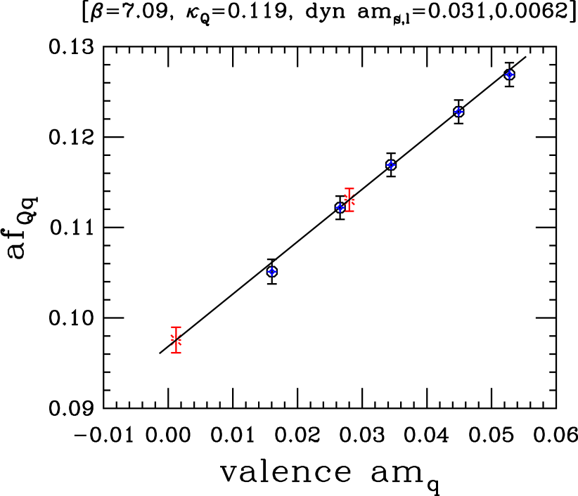
   Figure 1: Chiral extrapolation (interpolation) for $f_{B}$ ($f_{B_{s}}$) for $\beta=7.09$, $\kappa_{Q}=0.119$.

6. after removal of perturbative logarithms, fit $f_{Qq}\sqrt{M_{Qq}}$ to a power series in $1/M_{Qq}$ and interpolate to $B$, $B_{s}$, $D$ and $D_{s}$ meson masses

7. put the perturbative logarithm back and use the heavy-light axial-vector current renormalization constant to get the renormalized decay-constant

Just before the conference, we obtained the preliminary results of a perturbative calculation of the axial-vector renormalization constant $Z_{A}$ [5]. As these results are preliminary, and our use of the results has not been as thoroughly checked as we would like, the following results are to be considered preliminary. In particular, we have not yet tried tadpole improvement, which should help to determine the size of our systematic error. We note that when we reported on this calculation at Lattice 2002 [4], no perturbative or nonperturbative calculation of $Z_{A}$ was available. We used an ad hoc procedure based on comparison of our improved action quenched results with the continuum limit of earlier calculations using the Wilson gauge action and Wilson or Clover quarks. This was explained in more detail in Ref. [1].

After steps 1–7 are completed on each ensemble, we have a partially quenched result at a particular value of dynamical $m_{\pi}/m_{\rho}$. We then plot these results as a function of $(m_{\pi}/m_{\rho})^{2}$ to perform a chiral extrapolation for the sea quarks. Before looking at the decay constant of a specific meson, we note that if we plot the ratio of decay constants for two different mesons a good deal of the uncertainty from the renormalization constants and other systematic errors drops out. Figure 2 shows the ratio $f_{B_{s}}/f_{B}$ of meson decay constants. In Fig. 3, we show $f_{B_{s}}$.

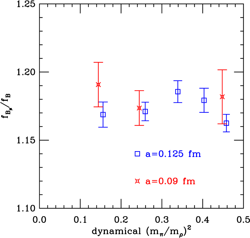
Figure 2: $f_{B_{s}}/f_{B}$ as a function of $(m_{\pi}/m_{\rho})^{2}$.

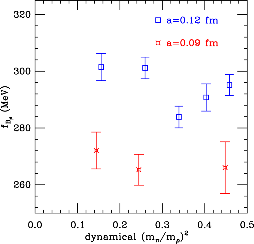
Figure 3: $f_{B_{s}}$ as a function of $(m_{\pi}/m_{\rho})^{2}$.

3 FUTURE WORK

We need to complete this analysis by including alternative cuts on the fits of meson propagators and alternative chiral extrapolations. We also must check the effect of tadpole improvement and see if we can employ a trick of Ref. [10] in which $Z_{A}^{hl}=\rho_{A}^{hl}\sqrt{Z_{V}^{hh}Z_{V}^{ll}}$ where $\rho_{A}^{hl}$ is computed perturbatively and both $Z_{V}$’s nonperturbatively. Although it would be possible to increase statistics on the fine configurations or include newer coarse ensembles ($a=0.12$ fm), our more recent effort with Asqtad light quarks appears to be more promising.

References

- [1] C. Bernard et al., Nucl. Phys. B (Proc. Suppl.) 106 (2002) 412.
- [2] A. El-Khadra, A. Kronfeld and P. Mackenzie, Phys. Rev. D55 (1997) 3933.
- [3] J. Simone et al., these proceedings.
- [4] C. Bernard et al., Nucl. Phys. B (Proc. Suppl.) 119 (2003) 613.
- [5] A. El Khadra, M. Nobes and H. Trottier, private communication.
- [6] G.P. Lepage, Phys. Rev. D59, (1999) 074502; K. Orginos, D. Toussaint and R.L. Sugar, Phys. Rev. D60, (1999) 054503.
- [7] C. Bernard et al., Phys. Rev. D64 (2001) 054506; C. Aubin et al., hep-lat/0402030, Phys. Rev. D to appear.
- [8] N. Yamada et al., Nucl. Phys. B (Proc. Suppl.) 106 (2002) 397; A.S. Kronfeld and S.M. Ryan, Phys. Lett. B543 (2002) 59; N. Yamada, Nucl. Phys. B (Proc. Suppl.) 119 (2003) 93.
- [9] C. Bernard et al., Phys. Rev. D66 (2002) 094501; D. Bećirević et al., Phys. Lett. B563 (2003) 150.
- [10] S. Hashimoto et al., Phys. Rev. D61 (2000) 014502.