Flavour singlet physics in lattice QCD with background fields

Abstract

We show that hadronic matrix elements can be extracted from lattice simulations with background fields that arise from operator exponentiation. Importantly, flavour-singlet matrix elements can be evaluated without requiring the computation of disconnected diagrams, thus facilitating a calculation of the quark contribution to the spin of the proton and the singlet axial coupling, $g_{A}^{0}$. In the two nucleon sector, a background field approach will allow calculation of the magnetic and quadrupole moments of the deuteron and an investigation of the EMC effect directly from lattice QCD. Matrix elements between states of differing momenta are also analysed in the presence of background fields.

The composition of the spin of the proton is a question of long-standing interest since experimentally it is known that only about 20% of the total spin of the proton is carried by the quark helicity spin . Contributions from quark orbital angular momentum and from gluon angular momentum are obviously important, but are currently unknown. Recently Ji Ji:1996ek has shown that a well-defined decomposition of the proton spin exists,

$$\frac{1}{2}=J_{q}+J_{g}=\frac{1}{2}\Sigma_{q}+L_{q}+J_{g}\,,$$ (1)

where each term is gauge invariant (though scheme and scale dependent) and given by proton matrix elements of the operators

$${\bf J}_{q} = \int d^{3}{\bf r}\,{\bf r}\times{\bf T}_{q}$$

$$= \frac{1}{2}\mbox{\boldmath$\Sigma$}_{q}+{\bf L}_{q}\equiv\int d^{3}{\bf r}\,\overline{\psi}\left[\frac{1}{2}\mbox{\boldmath$\gamma$}\gamma_{5}+\gamma_{0}{\bf r}\times(-i{\bf D})\right]\psi\,,$$

$${\bf J}_{g} = \int d^{3}{\bf r}\,{\bf r}\times({\bf E}\times{\bf B})\,,$$ (3)

where colour indices are suppressed, ${\bf T}_{q}^{j}=T_{q}^{j0}$ and $T_{q}^{\mu\nu}=\overline{\psi}\gamma^{\{\mu}i\tensor{D}^{\nu\}}\psi$ is the traceless, symmetric part of the quark energy-momentum tensor ($\tensor{D}=\frac{1}{2}[\roarrow{D}-\loarrow{D}]$). The quark helicity contribution, $\Sigma_{q}$, has been measured in polarised deep-inelastic scattering, but the separation of the quark orbital angular momentum and the total gluon angular momentum has not yet been determined from experiment though it can be extracted from deeply-virtual Compton scattering.

A reliable prediction of the various contributions to Eq. (1) from QCD would obviously be an important achievement. However, in QCD this question is non-perturbative since it involves hadronic-scale physics, and to address the issue from first principles, one must use lattice QCD. Indeed, proton matrix elements of both the helicity operator, $\overline{\psi}\gamma^{\mu}\gamma_{5}\psi$, lattice_gA0 ; lattice_helicity and the energy momentum tensor, $T^{\mu\nu}_{q}$, Mathur:1999uf ; Gadiyak:2001fe ; Hagler:2003jd ; Gockeler:2003jf have been computed and some estimates of the partitioning of the proton spin have been made. These calculations have been performed at unphysically large quark masses and on modest volumes and such parametric limitations make the connection of these results to the physical world non-trivial, though progress continues to be made in this regard ChPT ; Chen:2001pv ; Belitsky:2002jp ; FVGA ; FVTTMM . Such issues must be confronted for all hadronic quantities extracted from lattice simulations. However, the total quark helicity (singlet axial coupling) and angular momentum content of the proton are flavour singlet quantities ($g_{A}^{0}\sim\Sigma_{q}\sim\Sigma_{u}+\Sigma_{d}$ and $J_{q}\sim J_{u}+J_{d}$) and lattice calculations of them are further plagued by so-called quark-line disconnected contributions in which the relevant operator is inserted on a quark line connected to the proton source only by gluons as in Fig. 1(b). These terms are notoriously difficult to compute (see Ref. Gusken:1999te for a review) and result in relative errors an order of magnitude larger than the corresponding connected contributions.

Numerous other quantities such as the strangeness magnetic moment and the pion-nucleon sigma term suffer from the same difficulties. In the two nucleon sector, notable examples are the deuteron magnetic and quadrupole moments, and the deuteron structure function, $F_{2}^{d}(x)$, (accessible in lattice QCD only through two-particle matrix elements of twist-two operators EMCpaper ) that gives the simplest manifestation of the EMC effect Norton:2003cb . Even were it feasible to calculate five point correlators on present day computers, these quantities would again require orders of magnitude more computational effort than their flavour non-singlet analogues.

In this article, we highlight an alternative method to calculate operator matrix elements that eliminates the issue of disconnected contributions at the expense of requiring the generation of additional ensembles of gauge configurations. This essentially involves computing two-point correlators in the presence of generalised background fields which we show arise from exponentiating the operator whose matrix element we wish to calculate into the QCD action (see Ref. Fucito:ff for an early example). Since disconnected contributions are included automatically, this approach may provide a means of extracting reliable results for singlet matrix elements.

Electroweak background field methods have a long history in lattice QCD. In the early 1980s, Martinelli et al. Martinelli:1982cb and Bernard et al. Bernard:1982yu performed the first calculations of the magnetic moments of the proton, neutron and $\Delta$-resonance by calculating the baryon masses on a lattice immersed in a constant magnetic field. This approach has since been extended to calculate electric and magnetic polarisabilities of various hadrons Fiebig:1988en ; Christensen:2002wh ; Zhou:2002km ; Burkardt:1996vb . Fucito et al. Fucito:ff also showed that a background axial field could be used to determine the isovector axial coupling of the nucleon, $g_{A}$. Recently it has been demonstrated Detmold:2004qn that background electroweak fields can be used to probe the electroweak properties of two-nucleon systems. Measurement of two particle energy levels at finite volume in magnetic and weak background fields is sufficient to determine the weak- and magnetic- moments of the deuteron, and the threshold cross-sections for radiative capture ($n\,p\to d\gamma$) and weak-disintegration of the deuteron (e.g. $\nu_{x}d\to\nu_{x}n\,p$ $[x=e,\mu,\tau]$ and $\overline{\nu}_{e}d\to e^{+}n\,n$).

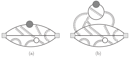
Figure 1: Connected (a) and quark-line disconnected (b) contributions to a baryon matrix element. The squares correspond to the baryon source and sink and the dark circle to the operator insertion.

In this work, we extend these analyses to consider more general background fields that correspond to exponentiation of a larger class of operators. We additionally consider the use of background fields to extract operator matrix elements between states of differing momenta. Such matrix elements determine the electromagnetic form-factors and moments of generalised parton distributions. Whilst much of the following analysis will be equally applicable in the pure-gauge and mesonic sectors, we restrict our discussion to baryons.

One baryon: In the single baryon sector, one is interested in calculating matrix elements of the form

$$\langle B^{\prime}({\bf p}^{\prime},s^{\prime})|{\cal O}|B({\bf p},s)\rangle\sim\overline{u}_{B^{\prime}}({\bf p}^{\prime},s^{\prime}){\cal M}_{B^{\prime}B}[{\cal O}]u_{B}({\bf p},s)\,,$$ (4)

where $q=p^{\prime}-p$ is the relative momentum of the baryons $B$ and $B^{\prime}$ ($s$ and $s^{\prime}$ label their spin) and $u_{B}({\bf p},s)$ is a baryon spinor. The Dirac structure ${\cal M_{B^{\prime}B}[{\cal O}]}$ is parameterised by a set of scalar form factors, $F_{i}(q^{2})$, depending on the particular operator, ${\cal O}$, and the external states (for the case of the energy-momentum tensor, we shall be more specific below). Typically, such form factors are calculated by computing ratios of two and three point correlators. We define

$$G_{BB}({\bf p},t;\Gamma)=\sum_{\bf x}e^{-i{\bf p}\cdot{\bf x}}\Gamma_{\beta\alpha}\langle 0|\chi^{(B)}_{\alpha}({\bf x},t)\overline{\chi}^{(B)}_{\beta}(0,0)|0\rangle\,,$$ (5)

and

$$G_{B^{\prime}{\cal O}B}({\bf p},{\bf p^{\prime}},t,\tau;\Gamma^{\prime}) = \sum_{{\bf x},{\bf y},{\bf z}}\Gamma^{\prime}_{\beta\alpha}e^{-i{\bf p}\cdot{\bf x}}e^{i{\bf p^{\prime}}\cdot{\bf z}}\langle 0|\chi^{(B^{\prime})}_{\alpha}({\bf x},t){\cal O}({\bf y},\tau)\overline{\chi}^{(B)}_{\beta}({\bf z},0)|0\rangle\,,$$ (6)

where $\Gamma$ and $\Gamma^{\prime}$ are Dirac projectors (the exact form of which depends on the operator under consideration), and $\chi_{\alpha}^{(B)}$ ($\overline{\chi}_{\beta}^{(B)}$) is an interpolating field for the baryon sink (source); for the proton, a common choice is $\chi^{(p)}_{\alpha}(x)=\epsilon_{ijk}u^{i}_{\alpha}(x)u^{j}_{\beta}(x)(C\gamma_{5})_{\beta\gamma}d^{k}_{\gamma}(x)$. It is easy to show (by inserting complete sets of states, see e.g. Ref Hagler:2003jd ) that the ratio

$$R({\bf p^{\prime}},{\bf p},t_{\rm sink},\tau;\Gamma,\Gamma^{\prime})=\frac{G_{B{\cal O}B}({\bf p^{\prime}},{\bf p},t_{\rm sink},\tau;\Gamma^{\prime})}{G_{BB}({\bf p^{\prime}},t_{\rm sink};\Gamma)}\,\left[\frac{G_{BB}({\bf p^{\prime}},\tau;\Gamma)G_{BB}({\bf p^{\prime}},t_{\rm sink};\Gamma)G_{BB}({\bf p},t_{\rm sink}-\tau;\Gamma)}{G_{BB}({\bf p},\tau;\Gamma)G_{BB}({\bf p},t_{\rm sink};\Gamma)G_{BB}({\bf p^{\prime}},t_{\rm sink}-\tau;\Gamma)}\right]^{1/2}\,,$$ (7)

will exhibit a plateau over a range of time slices $a\ll\tau\ll t_{\rm sink}$ where the sink time, $t_{\rm sink}$, is held fixed. For time slices within this plateau and appropriate choices of the Dirac projectors, this ratio is proportional to the form-factors under consideration. This approach and its variants (see e.g. Refs. Martinelli:1987bh ; Leinweber:1990dv ) are referred to as the operator insertion method. For flavour singlet operators, calculation of $G_{B{\cal O}B}$ requires evaluation of both types of diagram in Fig. 1.

For a local operator, ${\cal O}(z)$, at most bilinear in quark fields, it is possible to calculate the same matrix element by measuring a two-point correlator on an ensemble of field configurations generated with a modified Boltzmann weight. To see this, we add a term

$$\int d^{d}z\,{\cal O}(z)\cdot\Omega(z)\,,$$ (8)

to the usual QCD action, $S_{\rm QCD}$, with a fixed external source field $\Omega(z)$. If ${\cal O}(z)$, which depends on the quark ($\psi$) and gluon ($A_{\mu}$) fields and their derivatives, carries Lorentz or flavour indices, so does $\Omega(z)$. In the theory described by this action, the Euclidean space correlator of two baryon interpolating fields is given by:

$$\langle 0|{\chi}_{\alpha}(x)\overline{\chi}_{\alpha^{\prime}}(y)|0\rangle_{\Omega} = \frac{1}{{\cal Z}[\Omega]}\int{\cal D}A_{\mu}{\cal D}\psi{\cal D}\overline{\psi}{\chi}_{\alpha}(x)\overline{\chi}_{\alpha^{\prime}}(y)\exp\left(-S_{\rm QCD}[A,\psi,\overline{\psi}]-\int d^{d}z\;{\cal O}(z)\cdot\Omega(z)\right)$$

$$\xrightarrow{|\Omega|\to 0} \frac{1}{{\cal Z}[0]}\int{\cal D}A_{\mu}{\cal D}\psi{\cal D}\overline{\psi}{\chi}_{\alpha}(x)\overline{\chi}_{\alpha^{\prime}}(y)e^{-S_{\rm QCD}}\left[1+\frac{1}{{\cal Z}[0]}\int d^{d}z\Omega(z)\int{\cal D}A_{\mu}{\cal D}\psi{\cal D}\overline{\psi}{\cal O}(z)e^{-S_{\rm QCD}}\right]$$

$$\hskip 85.35826pt-\frac{1}{{\cal Z}[0]}\int d^{d}z\,\Omega(z)\int{\cal D}A_{\mu}{\cal D}\psi{\cal D}\overline{\psi}{\chi}_{\alpha}(x){\cal O}(z)\overline{\chi}_{\alpha^{\prime}}(y)e^{-S_{\rm QCD}}+{\cal O}(|\Omega|^{2})$$

$$= \langle 0|{\chi}_{\alpha}(x)\overline{\chi}_{\alpha^{\prime}}(y)|0\rangle_{0}\left[1+\int d^{d}z\,\Omega(z)\;\langle 0|{\cal O}(z)|0\rangle_{0}\right]-\int d^{d}z\,\Omega(z)\;\langle 0|{\chi}_{\alpha}(x){\cal O}(z)\overline{\chi}_{\alpha^{\prime}}(y)|0\rangle_{0}+{\cal O}(|\Omega|^{2})\,,$$

where ${\cal Z}[\Omega]$ is the partition function of the modified theory, $\langle\cdots\rangle_{\Omega}$ indicates a correlator evaluated in this theory, and $|\Omega|\to 0$ is a shorthand for requiring all tensor components of $\Omega(z)$ to be small compared to $\Lambda_{\rm QCD}^{{\rm dim}\,\Omega}$ (from Eq. (8), ${\rm dim}\,\Omega=d-{\rm dim}\,{\cal O}$). For operators for which $\langle 0|{\cal O}(z)|0\rangle=0$ [a notable exception being $\overline{\psi}(z)\psi(z)$], the (completely) disconnected contribution vanishes and we see that to leading order in the strength of the background field, $\Omega(z)$, the difference between the two-point correlators with $\Omega(z)=0$ and $\Omega(z)\neq 0$ is proportional to the form factors that we wish to extract. For example, defining the external field generalisation of Eq. (5) as

$$G_{B^{\prime}B}^{\Omega}({\bf p}^{\prime},{\bf p},t;\Gamma)=\sum_{{\bf x},{\bf y}}\Gamma_{\beta\alpha}e^{-i{\bf p}^{\prime}\cdot{\bf x}}e^{i{\bf p}\cdot{\bf y}}\langle 0|\chi^{(B^{\prime})}_{\alpha}({\bf x},t)\overline{\chi}^{(B)}_{\beta}({\bf y},0)|0\rangle_{\Omega}\,,$$ (10)

then

$$\frac{G_{BB}({\bf p},t;\Gamma)-G_{BB}^{\Omega}({\bf p},{\bf p},t;\Gamma)}{G_{BB}({\bf p},t;\Gamma)} \xrightarrow[|\Omega|\to 0]{t\to\infty} \frac{\widetilde{\Omega}(0)}{2\,E_{B}({\bf p})}\frac{{\rm tr}\left[\Gamma\left(-ip/+M_{B}\right){\cal M}_{BB}[{\cal O}]\left(-ip/+M_{B}\right)\right]}{{\rm tr}\left[\Gamma\left(-ip/+M_{B}\right)\right]}\,,$$ (11)

where $\widetilde{\Omega}(q)$ is the (discrete) Fourier transform of $\Omega(z)$, $M_{B}$ is the ground state baryon mass, $E_{B}({\bf p})=\sqrt{M_{B}^{2}+|{\bf p}|^{2}}$ and terms of ${\cal O}(|\Omega|^{2})$ are ignored. With appropriate choices of $\Gamma$, this gives the required form-factors at $q^{2}=0$. The non-forward case is discussed below.

If ${\cal O}(z)$ depends on quark fields, the effects of the external field will manifest themselves in the quark determinant and valence quark propagators after the fermionic functional integration is performed in Eq. (Flavour singlet physics in lattice QCD with background fields). In a lattice simulation where one approximates the integral over the field configurations by importance sampling, each choice of background field requires an additional ensemble of appropriately weighted gauge field configurations to be generated. We note that in quenched QCD a given set of gauge configurations can be modified to incorporate the effects of the exponentiated operator if it is composed of purely quark fields (such as the local electromagnetic and axial currents) as the operator and gauge field decouple in the absence of vacuum polarisation by dynamical sea quark loops. In more general cases, new gauge configurations are required even in the quenched theory.

This exponentiated operator (external field) method is exactly what has been used to calculate the quenched magnetic moment of the proton in Refs. Martinelli:1982cb ; Bernard:1982yu . Here the addition to the Lagrangian is given by

$${\cal O}^{\mu}_{EM}(z)=\overline{\psi}(z)\gamma^{\mu}\psi(z),\quad\Omega_{\mu}(z)=\frac{e\,B}{2}{\tiny\begin{pmatrix}-z_{2}\\ z_{1}\\ 0\\ 0\end{pmatrix}}\,,$$ (12)

producing a constant magnetic field in the $z_{3}$ direction over all lattice sites (ignore issues of periodicity at finite volume). In a lattice regularisation, the simplest local transcription of this current is not conserved and a multiplicative renormalisation factor is required; alternatively the lattice version of the conserved current Karsten:1980wd ; Martinelli:1987bh can be used. For small field strengths, $B$, differences Martinelli:1982cb ; Bernard:1982yu between correlators of spin-up and spin-down baryons then determine the relevant magnetic moment, $\mu_{B}$, since the lowest energy eigenstates behave as $M_{B}^{\pm}=M_{B}\pm\mu_{B}|B|+{\cal O}(|B|^{2})$ where $\pm$ refers to spin anti-aligned or aligned with the magnetic field. To extract the magnetic moment, one requires one set of pure QCD gauge configurations generated with $B=0$ to determine the mass, $M_{B}$, and another independent set of configurations generated with the modified action with $a|e\,B|\ll\Lambda_{\rm QCD}$ to determine the shifted masses, $M_{B}^{\pm}$. In practice, a few ensembles of configurations generated with different values of $B\neq 0$ may be needed to uniquely determine the mass shift linear in $B$.

The quark angular momentum contribution to the proton spin can be measured from a forward matrix element Gadiyak:2001fe in a background field since it can be defined as a spatial moment, ${\bf J}_{q}=\int d^{3}{\bf r}\;{\bf r}\times{\bf T}_{q}$ (as with the magnetic moment, $\mbox{\boldmath$\mu$}=\frac{1}{2}\int d^{3}{\bf r}\;{\bf r}\times{\bf j}^{EM}$ Jackson ); in the background field approach, one would add $\Omega$ times this integral to the QCD action and look at the shift in the exponential fall off of the two-point correlator exactly as for the magnetic moment. Since twist-two operators such as the energy-momentum tensor are not conserved even in the continuum, there is a multiplicative renormalisation factor that must be computed to obtain a final result. The renormalisation factors for various twist-two operators have been calculated Capitani:1994qn . A more generic approach not relying on moment equations (and hence valid for more general operators that cannot be written in such a form) can also be used to determine $J_{q}$. Nucleon matrix elements of the helicity independent, dimension four, twist-two quark operator take the form

$$\langle N({\bf p}^{\prime},s^{\prime})|\overline{\psi}_{f}\gamma^{\{\mu}i\tensor{D}^{\nu\}}\psi_{f}|N({\bf p},s)\rangle=\overline{u}_{N}({\bf p}^{\prime},s^{\prime})\Big{[}\gamma^{\{\mu}\overline{p}^{\nu\}}A_{f}(q^{2})-i\frac{q_{\rho}\sigma^{\rho\{\mu}}{2M}\overline{p}^{\nu\}}B_{f}(q^{2})+\frac{q^{\{\mu}q^{\nu\}}}{M}C_{f}(q^{2})\Big{]}u_{N}({\bf p},s)\,,$$ (13)

where $\overline{p}=\frac{1}{2}\left(p+p^{\prime}\right)$ and $\{\ldots\}$ indicates symmetrisation of indices and subtraction of traces. In terms of the form-factors, $A_{f}$, $B_{f}$ and $C_{f}$, the total quark angular momentum content for flavour $f$ is then given by Ji:1996ek $J_{f}=\frac{1}{2}\left[A_{f}(0)+B_{f}(0)\right]$. Since $B_{f}(q^{2})$ is always accompanied by a factor of the momentum transfer, the twist-two matrix elements must be calculated at $q\neq 0$ (using Eq. (7) for example) and then extrapolated to the forward limit. This necessarily leads to some uncertainty as the minimum available non-zero lattice momentum, $q_{\rm min}=2\pi/L$, is set by the lattice size, $L$. For current lattice simulations, $L\lesssim 3$ fm, so $q_{\rm min}\gtrsim 0.4$ GeV. Given such a large momentum extrapolation, the use of the spatial moment definition in Eq. (Flavour singlet physics in lattice QCD with background fields) within the background field approach may provide the cleanest determination of $J_{q}$.

Exponentiated operator methods can be used to calculate such off-forward matrix elements. To see this, we consider the following correlator (${\bf p}^{\prime}\neq{\bf p}$) in the presence of an exponentiated operator $\int d^{d}z\,\Omega(z)\cdot{\cal O}(z)$:

$$G_{B^{\prime}B}^{\Omega}({\bf p}^{\prime},{\bf p},t;\Gamma) = \sum_{{\bf x},{\bf y}}\Gamma_{\beta\alpha}e^{-i{\bf p}^{\prime}\cdot{\bf x}}e^{i{\bf p}\cdot{\bf y}}\langle 0|\chi^{(B^{\prime})}_{\alpha}({\bf x},\mbox{$\frac{t}{2}$})\overline{\chi}^{(B)}_{\beta}({\bf y},-\mbox{$\frac{t}{2}$})|0\rangle_{\Omega}$$

$$= -\sum_{{\bf x},{\bf y}}\sum_{{\bf z},\tau}\Gamma_{\beta\alpha}\Omega({\bf z},\tau)e^{-i{\bf p}^{\prime}\cdot{\bf x}}e^{i{\bf p}\cdot{\bf y}}\langle 0|\chi^{(B^{\prime})}_{\alpha}({\bf x},\mbox{$\frac{t}{2}$}){\cal O}({\bf z},\tau)\overline{\chi}^{(B)}_{\beta}({\bf y},-\mbox{$\frac{t}{2}$})|0\rangle+{\cal O}(|\Omega|^{2})$$

$$= -\sum_{n,{\bf p}_{n},s^{\prime}}\sum_{m,{\bf p}_{m},s}\sum_{{\bf x},{\bf y}}\sum_{{\bf z},\tau}\Gamma_{\beta\alpha}\Omega({\bf z},\tau)e^{-i\left({\bf p}_{n}-{\bf p}^{\prime}\right)\cdot{\bf x}}e^{i\left({\bf p}-{\bf p}_{m}\right)\cdot{\bf y}}e^{-i({\bf p}_{m}-{\bf p}_{n})\cdot{\bf z}}e^{-(E_{n}+E_{m})t/2}e^{(E_{n}-E_{m})\tau}$$

$$\hskip 56.9055pt\times\langle 0|\chi^{(B^{\prime})}_{\alpha}(0)|n,{\bf p}_{n},s^{\prime}\rangle\langle n,{\bf p}_{n},s^{\prime}|{\cal O}(0)|m,{\bf p}_{m},s\rangle\langle m,{\bf p}_{m},s|\overline{\chi}^{(B)}_{\beta}(0)|0\rangle+{\cal O}(|\Omega|^{2})$$

$$= -\sum_{n,m}e^{-(E_{n}+E_{m})t/2}\Gamma_{\beta\alpha}\sum_{s,s^{\prime}}\sum_{{\bf z},\tau}e^{-i({\bf p}-{\bf p}^{\prime})\cdot{\bf z}}e^{(E_{n}-E_{m})\tau}\Omega({\bf z},\tau)$$

$$\hskip 56.9055pt\times\langle 0|\chi^{(B^{\prime})}_{\alpha}(0)|n,{\bf p}^{\prime},s^{\prime}\rangle\langle n,{\bf p}^{\prime},s^{\prime}|{\cal O}(0)|m,{\bf p},s\rangle\langle m,{\bf p},s|\overline{\chi}^{(B)}_{\beta}(0)|0\rangle+{\cal O}(|\Omega|^{2})$$

$$\xrightarrow[|\Omega|\to 0]{t\to\infty} -e^{-\left[E_{B^{\prime}}+E_{B}\right]t/2}\sum_{s,s^{\prime}}\Gamma_{\beta\alpha}\widetilde{\Omega}(q)$$

$$\hskip 56.9055pt\times\langle 0|\chi^{(B^{\prime})}_{\alpha}(0)|B^{\prime}({\bf p}^{\prime},s^{\prime})\rangle\langle B^{\prime}({\bf p}^{\prime},s^{\prime})|{\cal O}(0)|B({\bf p},s)\rangle\langle B({\bf p},s)|\overline{\chi}^{(B)}_{\beta}(0)|0\rangle\,,$$

where $\widetilde{\Omega}(q)$ is again the (discrete) Fourier transform of $\Omega(z)$, $E_{B}$ and $E_{B^{\prime}}$ are the energies of the lowest $B$ and $B^{\prime}$ states with momentum ${\bf p}$ and ${\bf p}^{\prime}$. Since energy and momentum are conserved in pure QCD simulations, $G_{B^{\prime}B}^{0}({\bf p}^{\prime},{\bf p},t;\Gamma)\sim\delta_{B^{\prime}B}\delta^{3}({\bf p}^{\prime}-{\bf p})$. However, by including an external source that is inhomogeneous [$\Omega=\Omega({\bf z},\tau)$] in the action, energy and/or momentum can be injected through the operator coupled to the source and off-forward correlators can have non-zero values. By choosing appropriate external fields, the form factors implicit in ${\cal M}_{B^{\prime}B}[{\cal O}]$ are easily determined from

$$\frac{G_{B^{\prime}B}^{\Omega}({\bf p}^{\prime},{\bf p},t;\Gamma^{\prime})}{\sqrt{G_{B^{\prime}B^{\prime}}^{0}({\bf p}^{\prime},{\bf p}^{\prime},t;\Gamma)\,G_{BB}^{0}({\bf p},{\bf p},t;\Gamma)}}=-\frac{\widetilde{\Omega}(q)}{2\sqrt{M_{B}M_{B^{\prime}}}}\frac{{\rm tr}\left[\Gamma^{\prime}(-ip/^{\prime}+M_{B^{\prime}}){\cal M}_{B^{\prime}B}[{\cal O}](-ip/+M_{B})\right]}{\sqrt{{\rm tr}\left[\Gamma(-ip/^{\prime}+M_{B^{\prime}})\right]\,{\rm tr}\left[\Gamma(-ip/+M_{B})\right]}}+{\cal O}(|\Omega|^{2})\,,$$ (15)

with relevant choices of $\Gamma$ and $\Gamma^{\prime}$. The simplest choice would be an external field that is a plane wave, $\Omega(z)\sim\exp(-i\,\hat{q}\cdot z)$, such that $\widetilde{\Omega}(q)\sim\delta^{4}(q-\hat{q})$, but other choices are possible. Correlators in which both the source and sink momentum are fixed are easily computed Gockeler:1998ye .

This method will be applicable not only for off-forward matrix elements of the electromagnetic current (giving the Dirac and Pauli form factors) and the energy-momentum tensor (giving the form factors in Eq. (13)), but also for other quark bilinear operators. Important cases are the towers of twist-two operators ${\cal O}_{\Gamma,f}^{\mu_{0}\ldots\mu_{n}}=\overline{\psi}_{f}\Gamma^{\{\mu_{0}}i\tensor{D}^{\mu_{1}}\ldots i\tensor{D}^{\mu_{n}\}}\psi_{f}$ where $\Gamma^{\mu}=\gamma^{\mu},\,\gamma^{\mu}\gamma_{5},\,\sigma^{\alpha\mu}$ and $\{\ldots\}$ again indicates symmetrisation of indices and subtraction of traces. The non-forward matrix elements of these operators correspond to moments of generalised parton distributions (see Ref. Diehl:2003ny for a recent review). Finally we note that hadronic matrix elements of purely gluonic operators would also be accessible through the operator exponentiation approach but operators involving more than two quark fields cannot be exponentiated as they would prevent the fermionic functional integrals from being integrated exactly.

For many quantities the background field approach would not be particularly appealing as the added overhead (with respect to calculating a baryon two point correlator) of computing the quark propagators required in the standard three point correlator analysis is minimal as compared to the cost of generating additional ensembles of dynamical gauge configurations; particular examples are the moments of the isovector parton distribution functions. However, for flavour singlet quantities the situation may be reversed. In the operator insertion approach, one must evaluate the contributions of quark-line disconnected diagrams which are very difficult to compute as they involve propagators from all points on the lattice to themselves. Consequently, they require ensembles of gauge configurations that are an order of magnitude larger to achieve the same precision as in the corresponding connected diagrams Gusken:1999te even when stochastic estimator techniques Bitar:1988bb ; Dong:1993pk ; Eicker:1996gk ; Thron:1997iy ; Viehoff:1997wi ; Gusken:1998wy (which improve greatly on the brute force approach) are applied. In the background field approach, disconnected contributions are included automatically; for these calculations one requires a few additional, moderately sized ensembles of configurations generated with modified actions and this may be a more efficient means of calculating flavour singlet quantities. In terms of statistics and identification of the ground state, the external field method is somewhat similar to the plateau accumulation method Gusken:1998wy , but with the added advantage of automatically including quark-line disconnected diagrams. To extract physical quantities in either approach, calculations must be repeated at different quark masses, volumes and lattice spacings and then the necessary extrapolations must be performed. This may be more difficult using external fields than in the operator insertion approach where multi-mass techniques Frommer:1995ik are well developed (though similar techniques may also make the background field calculations easier). Numerical work to investigate the relative costs of the different approaches is encouraged.

Two baryons: In the two baryon sector, exponentiation of operators will also prove useful. It has recently been proposed that background electroweak fields can be used to measure the electroweak properties of two-nucleon states such as the deuteron magnetic moments and the cross-section for neutrino breakup of the deuteron Detmold:2004qn . For such two-hadron systems, even a calculation of the lowest energy levels involves large numbers of distinct Wick contractions and is only presently becoming feasible Fukugita:1994ve ; calculating matrix elements of such systems by an operator insertion is probably beyond the limits of current computational power. However, by measuring finite volume shifts in the low-lying two-particle energy levels in appropriate background fields, the various electroweak properties can be determined using effective field theory. Again, the exponentiated operator approach is especially suitable for flavour singlet quantities as disconnected diagrams, which would be required in the operator insertion approach, are included automatically. Provided one can construct deuteron interpolating fields that sufficiently project onto its different polarisations, similar background field methods will yield the quadrupole moment of the deuteron.

Another important phenomenon which background fields may prove useful in investigating is the modification of structure functions in nuclei – the EMC effect Norton:2003cb . The difference of the ratio $F_{2}^{d}(x)/\left[F_{2}^{p}(x)+F_{2}^{n}(x)\right]$ from unity is the simplest quantity in this regard (though experimentally the magnitude of the effect increases with atomic number). Important matrix elements that one might consider to investigate this on the lattice are $\langle N\,N|{\cal O}^{\mu_{0}\ldots\mu_{n}}_{\gamma,u+d}|N\,N\rangle$ EMCpaper since these determine the structure functions of two-nucleon states such as the deuteron via the operator product expansion. In a similar manner to the deuteron magnetic moment and neutrino-deuteron breakup cross-sections Detmold:2004qn , one can exponentiate the twist-two operators to create background fields. Then evaluating two-particle energy levels in these field and matching to effective field theory will enable calculation of the required matrix element. Again, since these matrix elements are isoscalar, the external field approach should be competitive with operator insertion techniques. Finally, we note that the same sets of generalised background field gauge configurations that one might use to calculate moments of twist-two operators in the single baryon and meson sectors would also be appropriate here.

In summary, background field methods in which an operator is exponentiated into the action are powerful tools for evaluating general hadronic matrix elements in lattice QCD. Here, we have highlighted some of the features of this approach. The method is not restricted to operators whose background fields have classical analogues; for example, twist-two operators, such as that determining the total angular momentum content of the proton, are ideal candidates. For flavour singlet matrix elements, disconnected diagrams are automatically calculated in the external field procedure, potentially leading to increased statistical precision in these quantities. The technique is also not limited to forward matrix elements; objects such as the electromagnetic form-factors and generalised parton distributions can also be computed with background fields. These advantages come at the cost of requiring additional ensembles of gauge configurations to be generated.

The author is grateful for discussions with C.-J. D. Lin, W. Melnitchouk, M. J. Savage, A. Shindler and J. M. Zanotti. This work is supported by the US Department of Energy under contract DE-FG03-97ER41014.

References

- (1) J. Ashman et al. [European Muon Collaboration], Nucl. Phys. B 328, 1 (1989); B. Adeva et al. [Spin Muon Collaboration], Phys. Lett. B 302, 533 (1993); P. L. Anthony et al. [E142 Collaboration], Phys. Rev. Lett. 71, 959 (1993); K. Abe et al. [E143 Collaboration], Phys. Rev. Lett. 75, 25 (1995). For a recent review, see B. W. Filippone and X. Ji, Adv. Nucl. Phys. 26, 1 (2001).
- (2) X. Ji, Phys. Rev. Lett. 78, 610 (1997).
- (3) R. Gupta and J. E. Mandula, Phys. Rev. D 50, 6931 (1994); M. Fukugita et al., Phys. Rev. Lett. 75, 2092 (1995); S. J. Dong, J. F. Lagaë and K. F. Liu, Phys. Rev. Lett. 75, 2096 (1995); S. Güsken et al., Phys. Rev. D 59, 114502 (1999); B. Alles et al., Nucl. Phys. Proc. Suppl. 63, 239 (1998).
- (4) M. Göckeler et al., Phys. Rev. D 53, 2317 (1996); M. Göckeler et al., Nucl. Phys. Proc. Suppl. 119, 32 (2003); D. Dolgov et al., Phys. Rev. D 66, 034506 (2002); S. Sasaki, K. Orginos, S. Ohta and T. Blum, Phys. Rev. D 68, 054509 (2003).
- (5) N. Mathur et al., Phys. Rev. D 62, 114504 (2000).
- (6) V. Gadiyak, X. Ji and C. Jung, Phys. Rev. D 65, 094510 (2002).
- (7) P. Hägler et al., Phys. Rev. D 68, 034505 (2003); P. Hägler et al., arXiv:hep-lat/0312014.
- (8) M. Göckeler et al., Phys. Rev. Lett. 92, 042002 (2004).
- (9) W. Detmold, et al., Phys. Rev. Lett. 87, 172001 (2001); D. Arndt and M. J. Savage, Nucl. Phys. A 697, 429 (2002); W. Detmold, W. Melnitchouk and A. W. Thomas, Phys. Rev. D 68, 034025 (2003); Phys. Rev. D 66, 054501 (2002); Eur. Phys. J. directC 3, 13 (2001); J. W. Chen and X. Ji, Phys. Lett. B 523, 107 (2001); J. W. Chen and M. J. Savage, Nucl. Phys. A 707, 452 (2002); Phys. Rev. D 65, 094001 (2002); S. R. Beane and M. J. Savage, Nucl. Phys. A 709, 319 (2002); Phys. Rev. D 68, 114502 (2003).
- (10) J. W. Chen and X. Ji, Phys. Rev. Lett. 88, 052003 (2002).
- (11) A. V. Belitsky and X. Ji, Phys. Lett. B 538, 289 (2002).
- (12) S. R. Beane and M. J. Savage, Phys. Rev. D 70, 074029 (2004); W. Detmold and M. J. Savage, Phys. Lett. B 599, 32 (2004).
- (13) W. Detmold and C.-J. D. Lin, arXiv:hep-lat/0501007.
- (14) S. Güsken, arXiv:hep-lat/9906034.
- (15) J. W. Chen and W. Detmold, arXiv:hep-ph/0412119.
- (16) P. R. Norton, Rept. Prog. Phys. 66, 1253 (2003).
- (17) F. Fucito, G. Parisi and S. Petrarca, Phys. Lett. B 115 (1982) 148.
- (18) G. Martinelli, G. Parisi, R. Petronzio and F. Rapuano, Phys. Lett. B 116, 434 (1982).
- (19) C. W. Bernard, T. Draper, K. Olynyk and M. Rushton, Phys. Rev. Lett. 49, 1076 (1982); C. W. Bernard, T. Draper and K. Olynyk, Nucl. Phys. B 220, 508 (1983).
- (20) H. R. Fiebig, W. Wilcox and R. M. Woloshyn, Nucl. Phys. B 324, 47 (1989).
- (21) J. Christensen et al., Nucl. Phys. Proc. Suppl. 119, 269 (2003); J. Christensen, W. Wilcox, F. X. Lee and L. Zhou, arXiv:hep-lat/0408024.
- (22) M. Burkardt, D. B. Leinweber and X. Jin, Phys. Lett. B 385, 52 (1996).
- (23) L. Zhou et al., Nucl. Phys. Proc. Suppl. 119, 272 (2003).
- (24) W. Detmold and M. J. Savage, Nucl. Phys. A 743 (2004), 170.
- (25) G. Martinelli and C. T. Sachrajda, Nucl. Phys. B 306, 865 (1988).
- (26) D. B. Leinweber, R. M. Woloshyn and T. Draper, Phys. Rev. D 43, 1659 (1991).
- (27) L. H. Karsten and J. Smit, Nucl. Phys. B 183, 103 (1981).
- (28) J. D. Jackson, Classical Electrodymanics, 2nd ed. (Wiley, New York, 1975).
- (29) W. Wilcox, Phys. Rev. D 66, 017502 (2002).
- (30) S. Capitani and G. Rossi, Nucl. Phys. B 433, 351 (1995); G. Beccarini et al., Nucl. Phys. B 456, 271 (1995); S. Capitani et al., arXiv:hep-lat/9711007; S. Capitani, Nucl. Phys. B 597, 313 (2001); A. Bucarelli, et al., Nucl. Phys. B 552, 379 (1999); F. Palombi, R. Petronzio and A. Shindler, Nucl. Phys. B 637, 243 (2002); M. Guagnelli et al., arXiv:hep-lat/0405027; Nucl. Phys. B 664, 276 (2003); A. Shindler et al., Nucl. Phys. Proc. Suppl. 129, 278 (2004); M. Göckeler et al., Nucl. Phys. B 544, 699 (1999).
- (31) P. F. Bedaque, Phys. Lett. B 593, 82 (2004).
- (32) M. Göckeler et al., Nucl. Phys. B 544, 699 (1999).
- (33) M. Diehl, Phys. Rept. 388, 41 (2003).
- (34) K. Bitar et al., Nucl. Phys. B 313, 348 (1989).
- (35) S. J. Dong and K.-F. Liu, Phys. Lett. B 328, 130 (1994).
- (36) N. Eicker et al., Phys. Lett. B 389, 720 (1996).
- (37) C. Thron, S. J. Dong, K. F. Liu and H. P. Ying, Phys. Rev. D 57, 1642 (1998).
- (38) J. Viehoff et al., Nucl. Phys. Proc. Suppl. 63, 269 (1998).
- (39) S. Güsken et al., Phys. Rev. D 59, 054504 (1999).
- (40) A. Frommer, B. Nockel, S. Güsken, T. Lippert and K. Schilling, Int. J. Mod. Phys. C 6, 627 (1995).
- (41) M. Fukugita et al., Phys. Rev. D 52, 3003 (1995).