Progress on a canonical finite density algorithm

Abstract

We test the finite density algorithm in the canonical ensemble which combines the HMC update with the accept/reject step according to the ratio of the fermion number projected determinant to the unprojected one as a way of avoiding the determinant fluctuation problem. We report our preliminary results on the Polyakov loop in different baryon number sectors which exhibit deconfinement transitions on small lattices. The largest density we obtain around $T_{c}$ is an order of magnitude larger than that of nuclear matter. From the conserved vector current, we calculate the quark number and verify that the mixing of different baryon sectors is small.

1 Motivation

The phase structure of QCD is relevant in the description of various phenomena: from subtle modifications of the cross-sections in high energy collisions of nuclei to exotic states of nuclear matter in neutron stars. Even though we have a good understanding of how to perform simulations at zero baryon density and finite temperature, the simulation with non-zero chemical potential has been problematic.

To deal with the complex phase that the chemical potential introduces to the fermion determinant, a number of techniques have been proposed: various reweighting methods, imaginary chemical potential, etc. They allow us to explore the phase structure at small values of the chemical potential and temperatures close to the critical temperature. All these methods have as a starting point the grand canonical partition function. We will present here an approach based on the canonical partition function which alleviates the sign problem, the overlap problem and the determinant fluctuation problems [1, 2]. Some preliminary results will also be reported.

2 Canonical partition function

The QCD canonical partition function with a fixed quark number can be constructed from the projection of the quark number from the determinant [3, 2]. The probability of having $k$ quark loops more than antiquark loops wrapping around the time direction in the loop expansion of a determinant is represented by the Fourier transform

$$P_{k}=\frac{1}{2\pi}\int_{0}^{2\pi}\mbox{d}\phi\,e^{-i\phi k}\det M_{\phi}.$$ (1)

where $\det M_{\phi}$ is the fermion determinant of the quark matrix with an additional U(1) phase $e^{i\phi}/e^{-i\phi}$ in the time forward/backward links on one time slice. Therefore, the canonical partition function can be written as

$$Z_{C}(k,T)=\int\mbox{\cal D}U\,e^{-S_{G}}\int_{0}^{2\pi}\frac{\mbox{d}\phi}{2\pi}e^{-i\phi k}\det M_{\phi}.$$ (2)

One can also derive this from the Fourier transform of the grand canonical partition function [4]

$$Z_{C}(k,T)=\int_{0}^{2\pi}\frac{\mbox{d}\phi}{2\pi}\,e^{-i\phi k}Z_{GC}(\mu_{q}=i\phi T,T)$$

To see this we can use the fugacity expansion of the grand canonical partition function

$$Z_{GC}(\mu_{q},T)=\sum_{k=-12V}^{12V}Z_{C}(k,T)e^{\mu_{q}k/T}$$ (3)

where $k=n_{q}-n_{\bar{q}}$ is the quark number and $\mu_{q}$ is the quark chemical potential. Using the usual expression for Lattice QCD grand canonical partition function, one obtains the same expression as in Eq. (2).

For Wilson fermions we can write $M_{\phi}(U)\equiv M(U_{\phi})=M(\mu=i\phi T,U)$ in terms of the standard fermion matrix

$$[M(U)]_{m,n} = \delta_{m,n}-\kappa(1-\gamma_{\mu})U_{\mu}(m)\delta_{m+\mu,n}$$

$$- \kappa(1+\gamma_{\mu})U^{\dagger}_{\mu}(n)\delta_{m,n+\mu}$$

and some modified gauge fields

$$(U_{\phi})_{\mu}(n)\equiv\left\{\begin{array}[]{ll}U_{\mu}(n)e^{-i\phi}&n_{4}=N_{t},\,\mu=4\\ U_{\mu}(n)&otherwise.\end{array}\right.$$ (6)

This should not be viewed as a change of the field variables but rather as a convenient way of writing the partition function. We should also note that although originally the phase $e^{-i\phi T}$ appears on all timelike links, we can accumulate it on the last time slice through a change of variables.

In order to evaluate the canonical partition function in Eq. (2) we need to replace the continuous Fourier transform with a discrete one. Using the discrete Fourier transform of the determinant

$$\mbox{det}_{k}M(U)\equiv\frac{1}{N}\sum_{n=0}^{N-1}e^{-ik\phi_{n}}\det M_{\phi_{n}}(U)$$

with $\phi_{n}=\frac{2\pi n}{N}$, we write the partition function as

$$\tilde{Z}_{C}(k)=\int\mbox{\cal D}U\,e^{-S_{G}(U)}\mbox{det}_{k}M(U)$$ (7)

This is the partition function that we will try to evaluate. The parameter $N$ defines the Fourier transform. In the limit $N\rightarrow\infty$ we recover the original partition function. For finite $N$ the partition function will only be an approximation of the canonical partition function. Using the fugacity expansion we can show that

$$\tilde{Z}_{C}(k)=\sum_{m=-\infty}^{\infty}Z_{C}(k+mN)$$

If $F_{B}$ denotes the baryon free energy we expect that

$$Z_{C}(N_{B})\propto e^{-|N_{B}|F_{B}/T},$$

in the confined phase. If this holds true then $\tilde{Z}_{C}(k)\approx Z_{C}(k)$ for $k\ll N$. However, this is an expectation that needs to be checked in our simulations.

3 Algorithm

To evaluate $\tilde{Z}_{C}(k)$ by Monte-Carlo techniques we need the integrand in (7) to be real and positive. Using the $\gamma_{5}$ hermiticity of the Wilson matrix it is easy to prove that $\det M(U_{\phi})$ is real. However, the integrand in (7) is the Fourier transform of the Wilson determinant. For $\mbox{det}_{k}M$ to be real we need that $\det M_{\phi}=\det M_{-\phi}$. From charge conjugation symmetry we know that $\langle\det M_{\phi}\rangle=\langle\det M_{-\phi}\rangle$. Unfortunately this relation doesn’t hold configuration by configuration. We are thus forced to remove the complex phase from $\mbox{det}_{k}M$.

To avoid dealing with the complex phase we will generate an ensemble using $|\mbox{Re}\,\mbox{det}_{k}M|$ as our probability function and we will then reintroduce the complex phase in observables. This is the standard way to deal with a complex phase in the weight function. It is also the source of the infamous sign problem. This might limit us in fully exploring the parameter space.

The focus of the algorithm will then be to generate an ensemble with the weight

$$W(U)=e^{-S_{G}(U)}\left|\frac{1}{N}\sum_{n=0}^{N-1}\cos(\phi_{n}k)\det M_{\phi_{n}}(U)\right|.$$

It was pointed out in [5] that taking the Fourier transform after the Monte Carlo simulations with different $\phi_{n}$ leads to an overlap problem. To avoid this problem, it was stressed [2, 1] that it is essential to perform the Fourier transform first to lock into one particular quark (or baryon) sector before the accept/reject step. The general approach is to break the updating process into two steps. In this case, one first uses an update for an approximate weight $W^{\prime}(U)$, and then use an accept/reject step to correct for the approximation. The efficiency of this strategy depends on how good the approximation is. For a poor approximation the acceptance rate in the second step will be very small.

One possible solution would be to update the gauge links using a heatbath for pure gauge action. In that case $W^{\prime}(U)=e^{-S_{G}(U)}$. However, it is known that such an updating strategy is very inefficient since the fermionic part is completely disregarded in the proposal step and the determinant, being an extensive quantity, can fluctuate wildly from one configuration to the next in the pure gauge updating process [6]. To avoid the overlap problem and the leading fluctuation in the determinant, it is proposed [1] to update using the HMC algorithm in the first step. For simplicity we will be simulating two degenerate flavors of quarks. This allows us to use the standard HMC update. In this case we have

$$W^{\prime}(U)=e^{-S_{G}(U)}\det M(U)$$

In the second step we have to accept/reject with the probability

$$P_{acc}=\min\left\{1,\omega(U^{\prime})/\omega(U)\right\}$$

where $\omega$ is the ratio of the weights

$$\omega(U)=\frac{W(U)}{W^{\prime}(U)}=\frac{|\mbox{Re}\,\mbox{det}_{k}M[U]|}{\det M[U]}.$$

Since $\mbox{det}_{k}M[U]$ and $\det M[U]$ are calculated on the same gauge configuration, we can write the determinant ratio as

$$\omega(U)=\frac{1}{N}\left|\sum_{n=0}^{N-1}\cos(\phi_{n}k)e^{Tr(\log M_{\phi_{n}}-\log M)}\right|.$$ (8)

The leading fluctuation in the determinant from one gauge configuration to the next is removed by the $Tr\log$ difference of the quark matrices of $M_{\phi_{n}}(U)$ and $M(U)$. This should greatly improve the acceptance rate compared to the case with direct accept/reject based on the $|\mbox{Re}\,\mbox{det}_{k}M(U)|$ itself.

4 Triality

The canonical partition function (2) has a $Z_{3}$ symmetry that is not present in the grand canonical partition function [7]. Under a transformation $U\rightarrow U_{\phi}$ where $U_{\phi}$ is defined as in (6) and $\phi=\pm\frac{2\pi}{3}$ we have

$$\mbox{det}_{k}M[U]\rightarrow\mbox{det}_{k}M[U_{\pm\frac{2\pi}{3}}]=e^{\pm i\frac{2\pi}{3}k}\mbox{det}_{k}M[U].$$

We see that when $k$ is a multiple of $3$ this transformation is a symmetry of the action. Incidentally, if this symmetry is not spontaneously broken the relation above guarantees that the canonical partition function will vanish for any $k$ that is not a multiple of $3$.

For $\tilde{Z}_{C}$, our approximation of the canonical partition function, to exhibit this symmetry we need to choose the parameter $N$ that defines the discrete Fourier transform to be a multiple of $3$.

Figure 1: Polyakov loop argument as a function of simulation time.

If N is a multiple of $3$ we have

$$W(U)=W(U_{\pm\frac{2\pi}{3}}).$$

However, the HMC weight $W^{\prime}$ does not respect this symmetry since $\det M$ is not symmetric under this transformation. In this case, our algorithm can become frozen for long periods of time. In Fig. 1 we show the argument of the Polyakov loop as a function of the simulation time. Under a $Z_{3}$ transformation $U\rightarrow U_{\pm\frac{2\pi}{3}}$ the argument of the Polyakov loop gets shifted by $\pm\frac{2\pi}{3}$. The HMC update strongly prefers the $0$ sector and when a tunneling occurs to one of the other sectors the accept/reject step will reject any change for a long period of time. Consequently the algorithm will be very poor in sampling the other sectors.

To alleviate this problem we will introduce a $Z_{3}$ hopping [8]. Since the weight $W$ is symmetric under this change we can intermix the regular updates with a change in the field variables $U\rightarrow U_{\pm\frac{2\pi}{3}}$, where we will choose the sign randomly (equal probability for each sign) to satisfy the detailed balance. This will decrease our acceptance by a factor of roughly $3$ but will sample all the $Z_{3}$ sectors in the same manner.

5 Simulation details

In order to simulate the ensemble given by the weight $W(U)$ we need to evaluate the Fourier transform of the determinant. Since the calculation of the determinant is quite time consuming we will need to use $N$ as small as possible. There is a proposal that employs an estimator for the determinant [9] but in this preliminary study we choose to calculate the determinant exactly using LU decomposition. We were thus limited to running on very small lattices, i.e. $4^{4}$, and with $N=12$. For each $\beta$ we run three simulations: one for $k=0$, one for $k=3$ and one for $k=6$. They correspond to $0$, $1$ and $2$ baryons in the box.

Table 1: The simulation parameters for our runs.

$\beta$	$a(\mbox{fm}$)	$m_{\pi}(\mbox{MeV})$	$V^{-1}(\mbox{fm}^{-3})$	$T(\mbox{MeV})$
5.1	0.35(3)	870(90)	0.36(12)	140(14)
5.2	0.31(2)	920(90)	0.52(17)	160(16)
5.3	0.24(2)	1050(100)	1.1(3)	205(20)

In order to get a reasonable box size we had to simulate at large lattice spacings. We used $\beta=5.1$, $5.2$ and $5.3$ with fixed $\kappa=0.158$. The relevant parameters can be found in Table 1. The lattice spacing is determined using standard dynamical action on a $12^{4}$ lattice for the same values of $\beta$ and $\kappa$. For the HMC part of the update we used trajectories of length $0.5$ with $\Delta\tau=0.01$. We adjusted the number of such trajectories between two consecutive accept/reject steps so that the acceptance stays within the $15\%$ to $30\%$ range. The configurations were saved after $10$ accept/reject steps. We collected about $100$ such configurations for each run.

6 Observables

As we mentioned earlier we need to reintroduce the phase when we compute the observables. For an observable $O$ we have the following expression

$$\langle O\rangle_{\tilde{Z}_{C}}=\frac{\langle O\alpha\rangle_{W}}{\langle\alpha\rangle_{W}}$$

where the subscript $\tilde{Z}_{C}$ stands for integration over the canonical ensemble given by (7), $W$ stands for the average over the weight $W$ and

$$\alpha\equiv\frac{\mbox{det}_{k}M}{|\mbox{Re}\,\mbox{det}_{k}M|}$$

is the reweighting phase. It is easy to see that the phase $\alpha$ should average, over an infinite ensemble, to a real number. This is direct consequence of the charge conjugation symmetry. The real part of this phase will always be $\pm 1$. This gives us a simple criterion to decide whether we have a sign problem; all we need to do is to check whether the phase has predominantly one sign. If the phase comes with plus and minus signs with close to equal probability then we have a sign problem. For our runs the data is collected in Table 2. We see that for $\beta=5.1$ and $k=6$ we are approaching the sign problem region.

Table 2: Average of real phase factor, $\langle\mbox{Re}\,\alpha\rangle_{W}$.

	k=0	k=3	k=6
$\beta$=5.1	1.00(0)	0.48(6)	0.17(10)
$\beta$=5.2	1.00(0)	0.61(8)	0.82(5)
$\beta$=5.3	1.00(0)	0.98(1)	0.96(3)

An interesting observable to measure is the Polyakov loop. Although the average value is expected to be zero due to the $Z_{3}$ symmetry, the distribution in the complex plane can tell us whether or not the symmetry is spontaneously broken. Usually the spontaneous breaking of the $Z_{3}$ symmetry is associated with deconfinement. In Fig. 2 we show the histograms of the Polyakov loop for our runs. We see that as we go from $\beta=5.2$ to $\beta=5.3$ the symmetry is broken even in the $k=0$ sector. This is the usual finite temperature phase transition at zero baryon density. According to Table 1 this happens somewhere between $160\,\mbox{MeV}$ and $205\,\mbox{MeV}$. This is somewhat higher than expected for dynamical simulations but can be explained in terms of our large quark masses. More interestingly, we see that under the critical temperature the transition still occurs as we increase the number of baryons. It is also apparent that as we lower $\beta$ ($\beta=5.1$), we are approaching a region where even the $N_{B}=1$ sector is confined.

Assuming that the result of $N_{B}=1(k=3)$ at $\beta=5.1$ is close to the phase transition line, the phase transition for $T=140\,\mbox{MeV}$ occurs at the baryon density of $0.36\,\mbox{fm}^{-3}$ which is about $2.3$ times the nuclear matter density. We see from Table 1 that there does not seem to be a problem of reaching a density an order of magnitude higher than that of the nuclear matter around $T_{c}$. For example, for $N_{B}=2(k=6)$ at $\beta=5.3$, the baryon density is $2.2(6)\,\mbox{fm}^{-3}$ which is $14$ times the nuclear matter density. However, we should not take these numbers seriously in view of the small volume and large quark mass in the present calculation (since the pion mass is $870\,\mbox{MeV}$ our quark mass is close to the strange quark one).

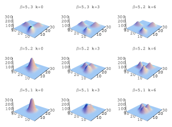
Figure 2: Polyakov loop distribution.

While it is nice to see that our expectation for the phase transition are confirmed in the gluonic sector, one would like to explore this transition in the fermionic sector too. It is important to note that the fermionic observables have to be evaluated in a non-standard manner. For example, if we are to study the fermionic bilinears we get

$$\langle\bar{\psi}\Gamma\psi\rangle = \frac{1}{Z_{C}}\frac{1}{N}\sum_{\phi}e^{-ik\phi}\int\mbox{\cal D}\bar{\psi}\mbox{\cal D}\psi e^{\bar{\psi}M_{\phi}\psi}\bar{\psi}\Gamma\psi$$

$$= \sum_{k^{\prime}}\frac{\mbox{det}_{k^{\prime}}M}{\mbox{det}_{k}M}(-\mbox{Tr}_{k-k^{\prime}}\Gamma M^{-1})$$

where

$$\mbox{Tr}_{k}\Gamma M^{-1}=\frac{1}{N}\sum_{\phi_{n}}e^{-ik\phi_{n}}\mbox{Tr}\Gamma M_{\phi_{n}}^{-1}.$$

We see that for fermionic variables, we need to do a Fourier transform on the observable too. We have measured the chiral condensate in our runs in the hope that it will signal chiral symmetry restoration. Unfortunately, it seems that the quarks are too heavy for us to get any signal. For example at $\beta=5.1$ and $\kappa=0.158$ we got $\langle\bar{\psi}\psi\rangle=-3.612(1)$, $-3.598(5)$ and $-3.601(2)$ for $N_{B}=0$, $1$ and $2$ respectively. We suspect that we need to lower the quark mass to be able to see any signal in the chiral condensate. Also, since we are working with Wilson fermions, the signal might be obscured by the mixing between $\bar{\psi}\psi$ and unity and other lattice artifacts especially at these large lattice spacings.

7 Sector mixing

It is important to note that all the calculations carried out above are using an approximation of the canonical partition function. As noted before it is an assumption on our part that $\tilde{Z}_{C}\approx Z_{C}$. To check this we measured the conserved charge for Wilson fermions

$$Q(t)=-\kappa\sum_{\vec{x}} [\bar{\psi}(x)U_{4}(x)(1-\gamma_{4})\psi(x+\hat{t})$$

$$-\bar{\psi}(x+\hat{t})U^{\dagger}_{4}(x)(1+\gamma_{4})\psi(x)].$$

The idea is that if we were to compute the conserved charge using the exact canonical ensemble $Z_{C}$ we would measure exactly the number of quarks we put it $\langle Q(t)\rangle_{Z_{C}(k)}=k$. However, in the discrete case we have

$$\langle Q(t)\rangle_{\tilde{Z}_{C}(k)}=\frac{\sum_{m}(k+mN)Z_{C}(k+mN)}{\sum_{m}Z_{C}(k+mN)}.$$

This is a weighted average over the various sectors allowed by our discretized delta function. If the approximation holds then the average of the conserved current should be closed to its exact value.

For $\beta=5.1$, we get the conserved charge to be $\langle Q(t)\rangle_{\tilde{Z}_{C}}=3.0004(4)$ for $k=3$ and $0$ for $k=0$ and $6$. We will first note that for $k=3$ we get the conserved charge to be very close to the exact value, indicating that there is very little mixing with the other allowed sectors $k=...-21,-9,15,27...$. The other two values are $0$ due to symmetry. For $k=0$ sector, it is easy to understand. For the $k=6$ sector, the explanation lies in the fact that $N=12$. Thus for every allowed sector $k+mN$ there is an $m^{\prime}$ such that $k+m^{\prime}N=-(k+mN)$. In that case the sum in the numerator vanishes and the conserved charge ends up being zero.

We conclude that there is very little mixing with the other allowed sectors in our runs. We attribute the smallness of the deviation in the case $k=3$ to the fact that the free energy for our baryons is very large. However, we expect that as we lower the quark mass the deviation will become more significant. If the deviation is too large then we might have to increase the parameter $N$ for the discrete Fourier transform.

8 Conclusions and outlook

Summing up, we showed that the canonical partition function approach can be used to investigate the phase structure of QCD. We are able to explore temperatures around the critical temperature and much higher densities than those available by other methods. We also find evidence that sign fluctuations might limit us in reaching much lower temperature and large fermion number. We checked that the discrete Fourier approximation to the canonical partition function introduces only minimal deviations.

In our runs, we find that even for a small lattice, the picture that emerges for the phase structure is consistent with expectations. The Polyakov loop shows signals of deconfining phase transition both in temperature and density directions. To complement this picture we would like to see a signal in the fermionic sector. For this we need to go to smaller masses and, maybe, to finer lattices.

Another goal would be to locate certain points on the phase transition line. For this we need to get to even lower temperatures and/or densities. While, we might be limited in going to much lower temperatures, we should be able to reach lower densities.

To reach a lower density with larger volume, we need to introduce an esitmator for the determinant. We should stress that the method used to generate the modified ensemble has no bearing on whether we have a sign problem or not. It is an intrinsic property of the modified ensemble. Consequently, we do not expect any difference in the sign behavior as we introduce the estimator.

References

- [1] K.F. Liu, Talk given at 3rd International Workshop on Numerical Analysis and Lattice QCD, Edinburgh, Scotland, 30 Jun - 4 Jul 2003, hep-lat/0312027.
- [2] K.F. Liu, Int. Jour. Mod. Phys.B16, 2017 (2002), hep-lat/0202026.
- [3] M. Faber, O. Borisenko, S. Mashkevich, and G. Zinovjev, Nucl. Phys. B444, 563 (1995).
- [4] E. Dagotto, A. Moreo, R. Sugar, and D. Toussaint, Phys. Rev. B41, 811 (1990); A. Hasenfratz and D. Toussaint, Nucl. Phys. B371, 539 (1992); J. Engels, O. Kaczmarek, F. Karsch, and E. Laermann, Nucl. Phys. B558, 307 (1999), hep-lat/9903030; M. Alford, A. Kapustin, and F. Wilczek, Phys. Rev. D59, 054502 (2000).
- [5] M. Alford, Nucl. Phys. B (Proc. Suppl.) 73, 161 (1999).
- [6] See for example B. Joo, I. Horvath, K. F. Liu, Phys. Rev. D67, 074505 (2003); A. Alexandru and A. Hasenfratz, Phys. Rev. D66, 094502 (2002).
- [7] M. Faber, O. Borisenko, S. Mashkevich, and G. Zinovjev, Nucl. Phys. B(Proc. Suppl.) 42, 484 (1995).
- [8] S. Kratochvila and P. de Forcrand, hep-lat/0309146.
- [9] C. Thron, S.J. Dong, K. F. Liu, and H. P. Ying, Phys. Rev. D57, 1642 (1998), hep-lat/9707001.