DESY 04-167
Edinburgh 2004/17
LTH 631
LU-ITP 2004/030
September 2004
Determination of Lambda in quenched and full QCD – an update

Abstract

We present an update on our previous determination of the Lambda parameter in QCD. The main emphasis is on results for two flavours of light dynamical quarks, where we can now almost double the amount of data used, including values at smaller lattice spacings. The calculations are performed using $O(a)$ improved Wilson fermions. Little change is found to previous numerical values.

The $\Lambda$ parameter is one of the fundamantal parameters of QCD, setting the scale for the running coupling constant $\alpha_{s}$. In this contribution we shall update our previous work, [1], both for quenched ($n_{f}=0$) and unquenched ($n_{f}=2$) $O(a)$ improved Wilson (‘clover’) fermions. Specifically we are now able to use for

• quenched fermions, the force scale $r_{0}/a$ up to $\beta=6.92$, [2] (previously $\beta\leq 6.4$),

• unquenched fermions, improved statistics and additional quark masses at the previous $\beta$ values of $5.20$, $5.25$, $5.29$ for $r_{0}/a$ together with new results at $\beta=5.40$ (at three quark masses).

The ‘running’ of the QCD coupling constant as the scale changes is controlled by the $\beta$-function

$${\partial g_{\cal S}(M)\over\partial\log M}=\beta^{\cal S}\left(g_{\cal S}(M)\right)\,,$$

where, perturbatively

$$\beta^{\cal S}\left(g_{\cal S}\right)=-b_{0}g_{\cal S}^{3}-b_{1}g_{\cal S}^{5}-b_{2}^{\cal S}g_{\cal S}^{7}-b_{3}^{\cal S}g_{\cal S}^{9}-\ldots\,,$$

renormalisation having introduced a scale $M$ together with a scheme $\cal S$. Integrating this equation gives

$${\Lambda^{\cal S}\over M} = \exp{\left[-{1\over 2b_{0}g_{\cal S}(M)^{2}}\right]}\left[b_{0}g_{\cal S}(M)^{2}\right]^{-{b_{1}\over 2b_{0}^{2}}}\times$$

$$\quad\exp{\left\{-\int_{0}^{g_{\cal S}(M)}d\xi\left[{1\over\beta^{\cal S}(\xi)}+{1\over b_{0}\xi^{3}}-{b_{1}\over b_{0}^{2}\xi}\right]\right\}}\,,$$

$$\equiv F^{\cal S}(g_{\cal S}(M))\,,$$

where $\Lambda^{\cal S}$, the integration constant, is the fundamental scheme dependent QCD parameter. Results are usually given in the $\overline{MS}$ scheme, with the scale $M$ being denoted by $\mu$. In this scheme the first four $\beta$-function coefficients are known, $b_{3}^{\mbox{\tiny$\overline{MS}$}}$ being found in [3]. The running coupling $\alpha^{\mbox{\tiny$\overline{MS}$}}_{s}(\mu)\equiv g_{\mbox{\tiny$\overline{MS}$}}(\mu)^{2}/4\pi$ is plotted in Fig. 1 for $n_{f}=2$, by solving

Figure 1: $\alpha_{s}^{\mbox{\tiny$\overline{MS}$}}(\mu)$ versus $\mu/\Lambda^{\mbox{\tiny$\overline{MS}$}}$ for $n_{f}=2$.

the previous equation (numerically) using successively more and more coefficients of the $\beta$-function. The figure shows an apparently fast convergent series (cf 3- to 4-loop), certainly in the range we are interested in, $\mu/\Lambda^{\mbox{\tiny$\overline{MS}$}}\sim 8$. A very similar result holds for $n_{f}=0$ but with slightly lower curves.

On the lattice we also have a $\Lambda$ parameter,

$$a\Lambda^{\Box}=F^{\Box}(g_{\Box}(a))\,,$$

where to help convergence of lattice perturbative expansions we use $g_{\Box}^{2}\equiv g^{2}(a)/u_{0}^{4}$ with $u_{0}^{4}$ the average plaquette value. To calculate $\Lambda^{\mbox{\tiny$\overline{MS}$}}$, we shall compute $g_{\mbox{\tiny$\overline{MS}$}}$ at some appropriate scale $\mu^{*}$ from $g_{\Box}(a)$ and then using the $r_{0}$ scale, extrapolate

$$r_{0}\Lambda^{\mbox{\tiny$\overline{MS}$}}\equiv\left(r_{0}\over a\right)F^{\mbox{\tiny$\overline{MS}$}}(g_{\mbox{\tiny$\overline{MS}$}}(\mu^{*}))a\mu^{*}\,,$$

to the continuum limit.

Equating lattice and continuum expressions

$$[F^{\mbox{\tiny$\overline{MS}$}}(g_{\mbox{\tiny$\overline{MS}$}}(\mu))]^{-1}=a\mu{\Lambda^{\Box}\over\Lambda^{\mbox{\tiny$\overline{MS}$}}}[F^{\Box}(g_{\Box}(a))]^{-1}\,,$$

and expanding as

$${1\over g_{\mbox{\tiny$\overline{MS}$}}^{2}(\mu)} = {1\over g_{\Box}^{2}(a)}+$$

$$[2b_{0}\ln a\mu-t^{\Box}_{1}]+[2b_{1}\ln a\mu-t^{\Box}_{2}]g_{\Box}^{2}(a)\ldots\,,$$

gives $t_{1}^{\Box}=2b_{0}\ln\Lambda^{\mbox{\tiny$\overline{MS}$}}/\Lambda^{\Box}$ and $b_{2}^{\Box}=b_{2}^{\mbox{\tiny$\overline{MS}$}}+b_{1}t^{\Box}_{1}-b_{0}t^{\Box}_{2}$. For (hopefully) good convergence of this series we choose the scale so that the $O(1)$ term vanishes, $a\mu^{*}=\exp(t_{1}^{\Box}/2b_{0})$.

For $t_{1}^{\Box}$ the general expression is known for $n_{f}$, $c_{sw}$ and linear terms in $n_{f}am_{q}$, while for $t_{2}^{\Box}$ the $n_{f}am_{q}$ dependence is not known, [1] and references therein. We can estimate the scales as $\mu^{*}=2.63/a$, $n_{f}=0$ and $\mu^{*}\sim 1.4/a$ for $n_{f}=2$. $t_{3}^{\Box}$ (the $g_{\mbox{\tiny$\overline{MS}$}}(\mu)^{4}$, $\ln a\mu$ independent term) is not known. So equivalently $b_{3}^{\Box}$ is not known. However a Padé estimate gives $b_{3}^{\cal S}\approx(b_{2}^{\cal S})^{2}/b_{1}$, and is small and in reasonable agreement with the known coefficient in the $\overline{MS}$ scheme, [1]. Assuming this also holds for $b_{3}^{\Box}$ gives little change to the results presented here. For complete $O(a)$ cancellation, [4], we need $\tilde{g}^{2}=g^{2}(1+b_{g}am_{q})$ where perturbatively $b_{g}=0.01200n_{f}g^{2}+O(g^{4})$, which with $c_{sw}=1+O(g^{2})$ then gives no mass dependence in $t_{1}^{\Box}$. This indicates little quark mass dependence in the fit formulae (indeed there is more in the numerical data). Finally to further improve the convergence of the series, we tadpole improve the $t_{i}^{\Box}$ coefficients $c_{sw}^{TI}=c_{sw}u_{0}^{3}$ (for $t_{1}^{\Box}+t_{2}^{\Box}g_{\Box}^{2}$) further reducing the size of the $n_{f}$ term in $t_{2}^{\Box}$.

In Fig. 2 we show the quenched ($n_{f}=0$) results.

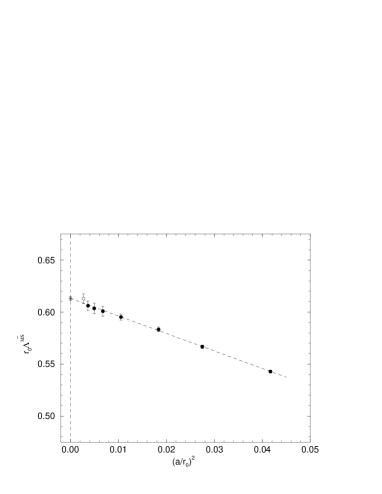
Figure 2: $r_{0}\Lambda^{\mbox{\tiny$\overline{MS}$}}$ versus $(a/r_{0})^{2}$ for $n_{f}=0$, together with a linear extrapolation to $a=0$. The last point has not been included in the fit.

The data lies on a straight line (as a function of $(a/r_{0})^{2}$) at least over $a^{-1}\sim 2$ – $6.5\,\mbox{GeV}$ or $\mu\sim 5$ – $17\,\mbox{GeV}$, using the value for $r_{0}$ of $r_{0}=0.5\,\mbox{fm}$. This gives a result of $r_{0}\Lambda^{\mbox{\tiny$\overline{MS}$}}=0.613(2)(25)$ or $\Lambda^{\mbox{\tiny$\overline{MS}$}}(0)=242(1)(10)\,\mbox{MeV}$ where the first error is statistical and to estimate the systematic uncertainty, the second error takes a $g^{4}\,\mbox{coeff.}=25\%\times g^{2}\,\mbox{coeff.}$ (which is very much greater than when using the Padé $b^{\Box}_{3}$ estimate).

For unquenched ($n_{f}=2$) fermions, due to the sea quark, the fit ansatz is not so simple as we must consider both chiral and continuum extrapolations. We take for finite $a$, $a\Lambda^{\mbox{\tiny$\overline{MS}$}}|_{m_{q}\not=0,a\not=0}=a\Lambda^{\mbox{\tiny$\overline{MS}$}}|_{m_{q}=0,a\not=0}+Dam_{q}+\ldots$ or $r_{0}\Lambda^{\mbox{\tiny$\overline{MS}$}}|_{m_{q}\not=0,a\not=0}=r_{0}\Lambda^{\mbox{\tiny$\overline{MS}$}}|_{m_{q}=0,a\not=0}+Dr_{0}m_{q}+\ldots$. After chiral extrapolation we would thus expect $r_{0}\Lambda^{\mbox{\tiny$\overline{MS}$}}|_{m_{q}=0,a\not=0}=r_{0}\Lambda^{\mbox{\tiny$\overline{MS}$}}|_{m_{q}=0,a=0}+B(a/\rho)^{2}+\ldots$ with $\rho\equiv r_{0}|_{m_{q}=0}$. Together with $(a/r_{0})^{2}=(a/\rho)^{2}+Eam_{q}+\ldots$ this gives our fit ansatz as

$$r_{0}\Lambda^{\mbox{\tiny$\overline{MS}$}}=A+B(a/r_{0})^{2}+Cam_{q}+Dr_{0}m_{q}\,.$$

So by subtracting out the $B$ and $C$ terms from $r_{0}\Lambda^{\mbox{\tiny$\overline{MS}$}}$ we can consider the chiral extrapolation and similarly by subtracting out the $C$ and $D$ terms we may consider the continuum extrapolation. In Fig. 3

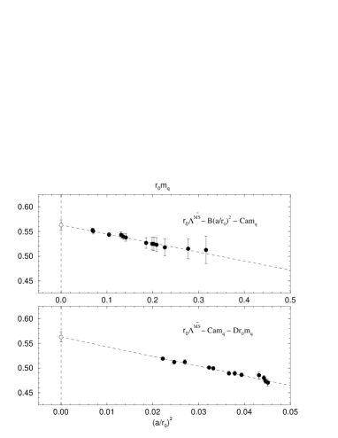
Figure 3: $r_{0}\Lambda^{\mbox{\tiny$\overline{MS}$}}$ versus $r_{0}m_{q}$ (upper picture) and versus $(a/r_{0})^{2}$ (lower picture) for $n_{f}=2$, together with appropriate extrapolations ($am_{q}$ from [5]).

we show the results. $a^{-1}$ ranges at least over $a^{-1}\sim 2$ – $3\,\mbox{GeV}$ or $\mu\sim 3$ – $4\,\mbox{GeV}$ This gives a result of $r_{0}\Lambda^{\mbox{\tiny$\overline{MS}$}}=0.563(10)(70)$ or $\Lambda^{\mbox{\tiny$\overline{MS}$}}(2)=222(4)(28)\,\mbox{MeV}$ where again the first error is statistical and the second error is obtained by taking a $g^{4}\,\mbox{coeff.}=25\%\times g^{2}\,\mbox{coeff.}$ which again is much larger than the error found when using a Padé $b^{\Box}_{3}$ estimate, setting $c_{sw}=1+O(g^{2})$ or including an additional $(am_{q})^{2}$ fit term. Note that this result is consistent with that obtained in [6].

Finally in Fig. 4 we present results for

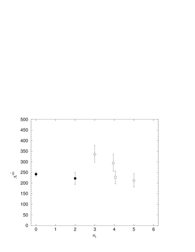
Figure 4: $\Lambda^{\mbox{\tiny$\overline{MS}$}}(n_{f})$ versus $n_{f}$ The open diamonds are from [7], using $\alpha_{s}^{\mbox{\tiny$\overline{MS}$}}(M_{Z})=0.1183(27)$ ($n_{f}=5$) to match to $n_{f}=4$ and $n_{f}=3$, while the open square is from [8]. The filled circles are the results reported here.

different $n_{f}$. Our result lies somewhat low in comparison with phenomenological results. Alternatively using the matching procedure as in [1] we find for $n_{f}=5$, $\alpha^{\mbox{\tiny$\overline{MS}$}}_{s}(m_{Z})=0.1084(6)(38)$.

References

[1]
S. Booth et al.,
Phys. Lett. B519 (2001) 229, hep-lat/0103023;
Nucl. Phys. Proc. Suppl.106 (2002) 308, hep-lat/0111006.
[2]
S. Necco et al.,
Nucl. Phys. B622 (2002) 328, hep-lat/0108008.
[3]
T. van Ritbergen et al.,
Phys. Lett. B400 (1997) 379, hep-ph/9701390.
[4]
M. Lüscher et al.,
Nucl. Phys. B478 (1996) 365, hep-lat/9605038.
[5]
M. Göckeler et al., in preparation.
[6]
G. Bali et al., hep-lat/0210033.
[7]
S. Bethke, hep-ex/0211012.
[8]
J. Blümlein et al.,
hep-ph/0407089.
[9]
C. R. Allton et al.,
Phys. Rev. D65 (2002) 054502, hep-lat/0107021.