Measuring interface tensions in ${\rm 4d}$ ${\rm SU(N)}$ lattice gauge theories

Abstract

We propose a new algorithm to compute the order-order interface tension in ${\rm SU(N)}$ lattice gauge theories. The algorithm is trivially generalizable to a variety of models, e.g., spin models. In the case $N=3$, via the perfect wetting hypothesis, we can estimate the order-disorder interface tension. In the case $N=4$, we study the ratio of dual $k-$tensions and find that it satisfies Casimir scaling down to $T=1.2~{}T_{c}$.

1 Introduction

The phenomenon of phase-coexistence is the typical signature of a first-order transition. The free energy of a system at the coexistence point is the sum of two contributions: the bulk free energy $F_{\rm bulk}$, scaling like the volume $V$, and the free energy $F_{\Sigma}$ of the interface $\Sigma$ separating the two bulk phases. $F_{\Sigma}$ scales like an area. The interface tension $\sigma$ is defined as $\sigma=\lim_{\Sigma\to\infty}\frac{F(\Sigma)}{\mid\Sigma\mid}$ (the reduced tension is defined as $\sigma^{R}=\frac{\sigma}{T}$). In the context of $SU(N)$ pure gauge theories ($N$ is the number of colors) phase-coexistence occurs in two different situations: one at $T\geq T_{c}$ between ordered phases pointing in different directions in color space, the other at $T_{c}$, between confined (‘disordered’) and deconfined (‘ordered’) phases. The corresponding interface tensions are indicated $\sigma_{\rm oo}$ and $\sigma_{\rm od}$ respectively.

This paper presents a new algorithm to measure the order-order interface tension. Nevertheless, we can also give an estimate of the order-disorder tension via the so-called perfect wetting hypothesis [1], which states that between two ordered phases a layer of disordered phase can be generated at no free energy cost. Therefore the free energy of one order-order interface is related to that of two order-disorder interfaces, namely $F_{\rm oo}=2F_{\rm od}$. In general, anyway, $\sigma_{\rm oo}=w\sigma_{\rm od},\hskip 2.84544ptw\leq 2$, because otherwise order-order interfaces would be unstable. Therefore the choice $w=2$ gives a lower bound for $\sigma_{od}$.

Our system is a $4d$ $SU(N)$ pure gauge theory at finite temperature with spatial periodic boundary conditions (b.c.). $a$ indicates the lattice spacing. The volume is $V=L^{3}\cdot L_{t}$; the Wilson action is used. We will indicate the elements of the center of $SU(N)$ by $\zeta_{i},\hskip 2.84544pti=1,\ldots,N$. Heat-bath and over-relaxation are applied to $SU(2)$ subgroups of the $SU(N)$ matrices, according to the strategy used in [2].

2 The method

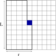
Figure 1: Cartoon of the interface, in an intermediate situation in which only half of the plaquettes has been flipped. The solid central plaquette is affected by the least finite size effects.

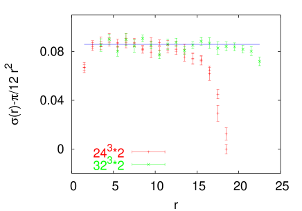
Figure 2: (Minus log of the) Ratios in Eq.(1) as a function of $r$, after removal of the Lüscher correction. A broad plateau develops from $r\sim\xi$ ($\xi=\frac{1}{\sqrt{\sigma}}\simeq 3.5$ is the correlation length) to $r\to L$.

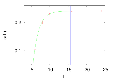
Figure 3: Finite size effects on the interface tension ($L_{t}=2$, $\beta=5.15$). After removal of the Lüscher correction, $\sigma$ is systematically underestimated, unless lattices larger than $L\gtrsim 7/\sqrt{\sigma}$ are used (vertical line). The curve is meant to guide the eye.

The algorithm we propose is an improvement of the so-called snake algorithm [3]. The ‘snake’ idea is to add ‘by hand’ a $2d$ interface in the system by progressively flipping the coupling of a set of plaquettes dual to a surface $A$, according to the identity

$$\frac{Z(A)}{Z(0)}=\frac{Z(A)}{Z(A-1)}\frac{Z(A-1)}{Z(A-2)}\ldots\frac{Z(1)}{Z(0)}$$ (1)

where $Z(k),\hskip 2.84544ptk\in[0,\ldots A]$ indicates the partition function of a system in which only $k$ plaquettes are flipped. The free energy of the interface is $F(A)=\sigma^{R}_{oo}A=-\log\frac{Z(A)}{Z(0)}$. A direct measurement of $\frac{Z(A)}{Z(0)}$ is not possible due to a serious overlap problem, which is alleviated by the factorization Eq.(1). The price to pay is a very large number ($L^{2}$) of independent simulations. Progress in this direction is made comparing the following equations

$$e^{-\sigma A}=\prod_{A}e^{-\sigma a^{2}},\qquad\frac{Z(A)}{Z(0)}=\prod_{A}\frac{Z(k)}{Z(k-1)}$$ (2)

the first just being a decomposition of the interface into the constituent plaquettes, the second indicating that each ratio, up to finite size (F.S.) corrections, contains all the information we need, namely

$$\frac{Z(k)}{Z(k-1)}=e^{-\sigma a^{2}}+(k-{\rm dependent\hskip 2.84544ptF.S.\hskip 2.84544ptcorrections})$$ (3)

so that a single simulation suffices. The gain in efficiency is ${\cal O}(L^{4})$: a factor $L^{2}$ in the number of simulations, another factor $L^{2}$ because the $L^{2}$ variances of the ratios add up in Eq.(1). The observable is measured in the following way:

$$\frac{Z(k)}{Z(k-1)}=\frac{\langle e^{\beta\frac{1}{3}{\rm Tr}(\zeta_{1}\Pi_{k})}\rangle_{k}}{\langle e^{\beta\frac{1}{3}{\rm Tr}(\Pi_{k})}\rangle_{k}}$$ (4)

where $\Pi_{k}$ indicates the $k-$th flipped plaquette, and the average $\langle\cdot\rangle_{k}$ refers to the ensemble in which the first $(k-1)$ plaquettes are flipped, the $k-$th plaquette has coupling zero, and all the others are unchanged. Further variance reduction methods are described in [3].

The leading finite-size corrections in Eq.(3) come from Gaussian fluctuations of the interface [4]. Our $r\cdot L$ interface (Fig. 1) is periodic in one direction ($L$), and pinned in the other ($r$). The corresponding correction, given in terms of the Dedekind $\eta$-function, reduces for $r\ll L$ to the Luscher-like $\sigma_{\rm eff}(r)\equiv-a^{-2}\log Z(k)/Z(k-1)\approx\sigma+\frac{\pi}{12r^{2}}$ [5]. In Fig. 2 we show our measurements, after removal of this known correction, as a function of $r$. A broad plateau develops, from small values $r\sim\xi$, where $\xi=1/\sqrt{\sigma}$ is the correlation length, to large ones $r\to L$, showing that additional corrections are very small. At very large distances, a systematic drop is visible, because it becomes more favorable to produce a full, translationally invariant interface plus a partial one of width $(L-r)$. Let us then fix $r=(\frac{L}{2}-1)$; after removal of the Lüscher corrections, Fig. 3 shows that the tension decreases considerably with the lattice size and reaches a plateau only when the empirical condition $L\sqrt{\sigma}\gtrsim 7$ is satisfied.

3 Results

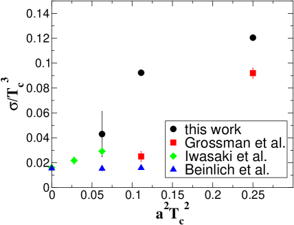
Figure 4: Summary of results on the order-disorder interface tension for $SU(3)$. To avoid an underestimate of $\sigma$ because of F.S. effects, we use a lattice of size $32^{3}\cdot 2$ ($a^{2}T_{c}^{2}=1/4$), $48^{3}\cdot 3$ ($a^{2}T_{c}^{2}=1/9$), $64^{3}\cdot 4$ $(a^{2}T_{c}^{2}=1/16)$. The latter simulation is in progress.

In Fig. 4 we present preliminary results for the order-disorder interface tension in $SU(3)$, together with a compilation of the published data. While our $L_{t}=4$ simulation needs more statistics, our $L_{t}=2$ and $3$ determinations of $\sigma$ are accurate, and much larger than previous measurements obtained with the histogram method [6][7][8][9]. We assign this discrepancy to the smaller lattice sizes considered previously, which lead to a systematic underestimate of $\sigma$ as in Fig. 3. A discussion of the continuum limit is awaiting completion of the $64^{3}\cdot 4$ simulations.

$T/T_{c}$	$L=16$	$L=24$
2.3	1.350(20)	1.342(13)
1.5	-	1.300(18)
1.2	1.277(33)	1.310(30)

Table 1: Ratio $\sigma_{2}/\sigma_{1}$ of $SU(4)$ interface tensions ($L_{t}=5$). The Casimir perturbative value is $4/3$. For the data at $T=1.2~{}T_{c}$ we find again that the F.S. effects are smaller than the statistical error only if $L\gtrsim 7/\sqrt{\sigma}$.

In Tab.1 we present preliminary results for the case $SU(4)$. In $SU(N)$ with $N>3$ we have more order-order tensions ($\sigma_{k},\hskip 1.42271ptk=1,\ldots,[N/2]$). In the weak coupling regime one can show the Casimir relation $\frac{\sigma_{k}}{\sigma_{1}}=\frac{k(N-k)}{N-1}$ [10]. This perturbative prediction seems accurate down to temperature $T=1.2~{}T_{c}$. Measurements closer to $T_{c}$ are in progress.

References

- [1] Z. Frei and A. Patkos, Phys. Lett. B 229, 102 (1989).
- [2] N. Cabibbo and E. Marinari, Phys. Lett. B 119, 387 (1982).
- [3] P. de Forcrand, M. D’Elia and M. Pepe, Phys. Rev. Lett. 86, 1438 (2001) [arXiv:hep-lat/0007034].
- [4] M. Luscher, Nucl. Phys. B 180, 317 (1981).
- [5] K. Dietz and T. Filk, Phys. Rev. D 27, 2944 (1983).
- [6] Y. Iwasaki, K. Kanaya, L. Karkkainen, K. Rummukainen and T. Yoshie, Phys. Rev. D 49, 3540 (1994) [arXiv:hep-lat/9309003].
- [7] B. Grossmann, M. L. Laursen, T. Trappenberg and U. J. Wiese, Nucl. Phys. Proc. Suppl. 30, 869 (1993) [arXiv:hep-lat/9210041].
- [8] B. Beinlich, F. Karsch and A. Peikert, Phys. Lett. B 390, 268 (1997) [arXiv:hep-lat/9608141].
- [9] A. Papa, Phys. Lett. B 420, 91 (1998) [arXiv:hep-lat/9710091].
- [10] P. Giovannangeli and C. P. Korthals Altes, Nucl. Phys. B 608, 203 (2001) [arXiv:hep-ph/0102022].