CP^N-1 model with the theta term and maximum entropy method

Abstract

A $\theta$ term in lattice field theory causes the sign problem in Monte Carlo simulations. This problem can be circumvented by Fourier-transforming the topological charge distribution $P(Q)$. This strategy, however, has a limitation, because errors of $P(Q)$ prevent one from calculating the partition function ${\cal Z}(\theta)$ properly for large volumes. This is called flattening. As an alternative approach to the Fourier method, we utilize the maximum entropy method (MEM) to calculate ${\cal Z}(\theta)$. We apply the MEM to Monte Carlo data of the CP³ model. It is found that in the non-flattening case, the result of the MEM agrees with that of the Fourier transform, while in the flattening case, the MEM gives smooth ${\cal Z}(\theta)$.

1 INTRODUCTION

It is well known that QCD in principle has a $\theta$ term. The $\theta$ term is deeply associated with non-perturbative properties of QCD at low energy and provides us with interesting issues such as the strong CP problem, possibilities of rich phase structures in $\theta$ space and so on. So it is a challenging subject to investigate the dynamics of QCD with the $\theta$ term.

The $\theta$ term in lattice field theory makes the Boltzmann weight complex and prevents one from performing Monte Carlo (MC) simulations directly. This is the sign problem. This problem can be circumvented by Fourier-transforming the topological charge distribution[1, 2, 3]

$$P(Q)\equiv\frac{\int[{\cal D}\phi]_{Q}\;e^{-S(\phi)}}{\int{\cal D}\phi\;e^{-S(\phi)}},$$ (1)

where $Q,\;\phi\;{\mbox{\rm and}}\;S$ are the topological charge, a field of the system and an action, respectively. The measure $[{\cal D}\phi]_{Q}$ implies that the integral is restricted to configurations of $\phi$ with $Q$. The partition function is given in terms of $P(Q)$ by

$${\cal Z}(\theta)=\sum_{Q}P(Q)e^{i\theta Q}.$$ (2)

Although this method works well for small volumes, it does not work for large ones because errors of $P(Q)$ affect strongly the behavior of the free energy density, $f(\theta)\equiv-\frac{1}{V}\log{\cal Z}(\theta)$ ($V$ is a volume). This is called flattening[4, 5]. Flattening can be remedied by reducing the errors, but this is hopeless, because exponentially increasing statistics are needed as volume increases.

In order to deal with flattening, we have utilized the maximum entropy method (MEM)[6, 7, 8]. In ref.[9], we applied the MEM to mock data of the Gaussian $P(Q)$ to study whether the MEM is effective to our issue. In the non-flattening case, the MEM reproduces the exact ${\cal Z}(\theta)$, while it gives smooth ${\cal Z}(\theta)$ in the case where flattening occurs in the Fourier method. In the present work, as the next step, we apply the MEM to MC data of the CP^N-1 model, which has several dynamical properties in common with QCD.

2 FLATTENING AND MEM

We simulated the CP³ model with a fixed point action at a fixed coupling constant, $\beta=3.0$[3]. The lattice extension $L$ is changed from 4 to 96. The statistics are more than 1 million for each case.

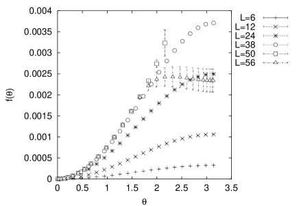
Figure 1: Free energy density $f(\theta)$ of the MC data of the CP³ model. Lattice extension $L$ of the system is changed from 6 to 56.

Figure 1 displays $f(\theta)$ obtained numerically by Fourier-transforming $P(Q)$ of the MC data for various volumes. Up to $L=38$, the Fourier transform works, but $f(\theta)$ for $L=50$ and 56 cannot be calculated properly. Especially for $L=56$, $f(\theta)$ becomes flat for $\theta\hskip 3.00003pt\raisebox{1.72218pt}{$>$}\raisebox{-3.01385pt}{$\sim$}\hskip 3.00003pt2.0$. This is nothing but flattening. The density $f(\theta)$ for $L=50$ breaks down for $\theta\hskip 3.00003pt\raisebox{1.72218pt}{$>$}\raisebox{-3.01385pt}{$\sim$}\hskip 3.00003pt2.3$ due to the negative values of ${\cal Z}(\theta)$. We also call it flattening because errors of $P(Q)$ disturb the behavior of $f(\theta)$.

In order to deal with flattening, we employ the MEM. To this end, we utilize the inverse Fourier transform. The MEM is based on Bayes’ theorem and gives the most probable image of ${\cal Z}(\theta)$. In our case, the most important object is the posterior probability ${\rm prob}({\cal Z}(\theta)|P(Q),I)$ which is the probability that ${\cal Z}(\theta)$ is realized when the MC data of $\{P(Q)\}$ and information $I$ are given. Information $I$ represents our state of knowledge about ${\cal Z}(\theta)$. Here we impose the criterion ${\cal Z}(\theta)>0$.

The probability ${\rm prob}({\cal Z}(\theta)|P(Q),I)$ is represented in terms of $\chi^{2}$ and the entropy $S$:

$${\rm prob}({\cal Z}(\theta)|P(Q),I)\propto\exp\biggl{[}-\frac{1}{2}\chi^{2}+\alpha S\biggr{]},$$ (3)

where $\alpha$ is a real positive parameter. Conventionally the Shannon-Jaynes entropy is employed;

$$S=\int_{-\pi}^{\pi}d\theta\biggl{[}{\cal Z}(\theta)-m(\theta)-{\cal Z}(\theta)\log\frac{{\cal Z}(\theta)}{m(\theta)}\biggr{]},$$ (4)

where $m(\theta)$ is called the default model and is chosen so as to be consistent with information $I$. To sum up, our task is to calculate the most probable image ${\hat{\cal Z}}(\theta)$ such that ${\rm prob}({\cal Z}|P(Q),I)$ is maximized( see refs.[8, 9] for details).

3 RESULTS

We apply the MEM to such MC data that flattening occurs in the Fourier method as well as to such MC data that it does not. Here we use the MC data for $L=38$(data A) as an example of the non-flattening case and for $L=50$(data B) for the flattening one. Two types of default model are used: (i) Gaussian type, $m_{G}(\theta)=\exp\bigl{[}-\gamma\frac{\log 10}{\pi^{2}}\theta^{2}\bigr{]}$, where a parameter $\gamma$ is changed from 0.6 to 5.0. (ii) weak coupling region type, $m_{\rm w}(\theta)$, which will be explained later. In the analysis, the Newton method with quadruple precision is used to calculate an image ${\hat{\cal Z}}(\theta)$ with high precision.

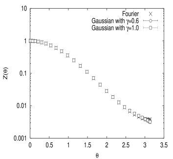
Figure 2: The most probable image ${\hat{\cal Z}}(\theta)$ of the MC data for $L=38$. The Gaussian type default models with $\gamma=0.6$ and 1.0 are used. As a comparison, the result of the Fourier transform($\times$) is also displayed.

Figure 2 displays the most probable image ${\hat{\cal Z}}(\theta)$ of data A, as an example of the non-flattening case. The Gaussian type default models $m_{G}(\theta)$ with $\gamma=0.6$ and 1.0 are used. The partition function ${\cal Z}(\theta)(\equiv{\cal Z}_{F}(\theta))$ obtained by Fourier-transforming $P(Q)$ of data A is also displayed. The result of the MEM agrees with that of the Fourier transform in the whole $\theta$ region. Note that errors of ${\hat{\cal Z}}(\theta)$ are too small to be visible, where the error of ${\hat{\cal Z}}(\theta)$ means the uncertainty of ${\hat{\cal Z}(\theta)}$[7, 8].

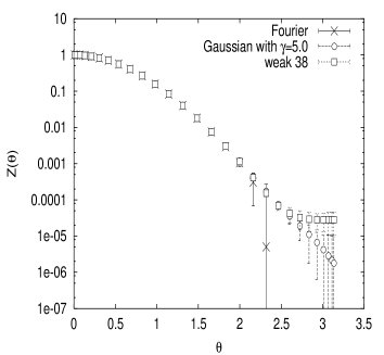
Figure 3: The most probable image ${\hat{\cal Z}}(\theta)$ of the MC data for $L=50$. Two types of default model are used. The result of the Fourier transform($\times$) is also displayed.

Next, let us turn to the data B, the flattening case. The results are shown in Fig. 3. The partition function ${\cal Z}_{F}(\theta)$ of data B breaks down for $\theta\hskip 3.00003pt\raisebox{1.72218pt}{$>$}\raisebox{-3.01385pt}{$\sim$}\hskip 3.00003pt2.3$ because the values of ${\cal Z}_{F}(\theta)$ become negative in this region. For the MEM analysis, the Gaussian type $m_{G}(\theta)$ with $\gamma=5.0$ and the weak coupling region type $m_{\rm w}(\theta)$ are used. Since $P(Q)$ of data A was successfully Fourier-transformed to ${\cal Z}(\theta)\equiv{\cal Z}_{A}(\theta)$, we use ${\cal Z}_{A}(\theta)$ as $m_{\rm w}(\theta)$ for the analysis of data for larger volumes. The results of the MEM reproduce smooth ${\hat{\cal Z}}(\theta)$ in the whole $\theta$ region. For $\theta\hskip 3.00003pt\raisebox{1.72218pt}{$>$}\raisebox{-3.01385pt}{$\sim$}\hskip 3.00003pt2.7$ they depend on the default models and give no definite solution about the behavior of ${\cal Z}(\theta)$ for $\theta\simeq\pi$ due to the large magnitude of the errors. For $\theta\hskip 3.00003pt\raisebox{1.72218pt}{$<$}\raisebox{-3.01385pt}{$\sim$}\hskip 3.00003pt2.7$, however, the results of the MEM show no $m(\theta)$-dependence and their errors are small. We thus obtain a reasonably good solution of ${\cal Z}(\theta)$ for $L=50$ up to $\theta=2.7$, which is wider than the valid region of the Fourier method.

4 SUMMARY

We applied the MEM to the MC data of the CP³ model for various volumes. It was found that the MEM is applicable to the CP³ model in the non-flattening and the flattening cases, and that the MEM has the advantage of calculating ${\cal Z}(\theta)$ for somewhat wider $\theta$ region than the Fourier transform at least for $L=50$. The following subjects remain to be investigated; (i) a systematic study of the $m(\theta)$-dependence of ${\hat{\cal Z}}(\theta)$ and its error, (ii) investigation on a question whether the MEM is more effective than the Fourier method, and (iii) a study of the feasibility of distinction between flattening and the signal of a first order phase transition[10].

References

- [1] G. Bhanot, E. Rabinovici, N. Seiberg and P. Woit, Nucl. Phys. B230[FS10] (1984), 291.
-
[2]
U. -J. Wiese, Nucl. Phys. B318 (1989), 153.
W. Bietenholz, A. Pochinsky and U. -J. Wiese, Phys. Rev. Lett. 75 (1995), 4524. - [3] R. Burkhalter, M. Imachi, Y. Shinno and H. Yoneyama, Prog. Theor. Phys. 106 (2001), 613.
- [4] J. C. Plefka and S. Samuel, Phys. Rev. D56 (1997), 44.
- [5] M. Imachi, S. Kanou and H. Yoneyama, Prog. Theor. Phys. 102 (1999), 653.
- [6] R. K. Bryan, Eur. Biophys. J. 18 (1990), 165.
- [7] M. Jarrell and J. E. Gubernatis, Phys. Rep. 269 (1996), 133.
- [8] M. Asakawa, T. Hatsuda and Y. Nakahara, Prog. Part. Nucl. Phys. 46 (2001), 459.
- [9] M. Imachi, Y. Shinno and H. Yoneyama, Prog. Theor. Phys. 111 (2004), 387.
- [10] M. Imachi, Y. Shinno and H. Yoneyama, poster at this conference.