Abstract

The effect of repeatedly smearing $SU(3)$ gauge configurations is investigated. Six gauge actions (Wilson, Symanzik, Iwasaki, DBW2, Beinlich-Karsch-Laermann, Langfeld; combined with a direct $SU(3)$-overrelaxation step) and three smearings (APE, HYP, EXP) are compared. The impact on large Wilson loops is monitored, confirming the signal-to-noise prediction by Lepage. The fat-link definition of the “naive” topological charge proves most useful on improved action ensembles.

1 Introduction

Smearing of gauge-links has been used on many occasions as a powerful tool to reduce the UV-fluctuations of a gauge configuration [2, 3, 4, 5, 6]. In principle, such a UV-filtering may be attempted either in the Monte Carlo process itself (by complementing the action with contributions from $W^{1\times 2+2\times 1}$ and even larger Wilson loops) or in the observable (where replacing the original links by smeared ones is just the simplest way to define a filtered observable). Normally, the motivation for the first option is not to tame the noise in standard observables, but to reduce cut-off effects. Nonetheless, an obvious question is whether there is an interplay between the action used to generate a pure gauge ensemble and the effectiveness of a smearing recipe to decrease the UV-fluctuations in a given observable.

	1	2	3	4	1	2	3	4	1	2	3	4
1	$\!0.5937\!$				$\!0.9509\!$				$\!0.0399\!$
2	$\!0.3836\!$	$\!0.1902\!$			$\!0.9015\!$	$\!0.7551\!$			$\!0.0073\!$	$\!0.0011\!$
3	$\!0.2527\!$	$\!0.1014\!$	$\!0.0471\!$		$\!0.8399\!$	$\!0.6205\!$	$\!0.4551\!$		$\!0.0013\!$	$\!0.0002\!$	$\!0.0000\!$
4	$\!0.1673\!$	$\!0.0553\!$	$\!0.0229\!$	$\!0.0101\!$	$\!0.7843\!$	$\!0.5149\!$	$\!0.3416\!$	$\!0.2357\!$	$\!0.0002\!$	$\!0.0000\!$	$\!0.0000\!$	$\!0.0000\!$

Table 1: Wilson loops $\langle W(R,T)\rangle$ with $R,T\in\{1,...,4\}$ on a $12^{4}$ lattice with Wilson glue at $\beta\!=\!6.0$ (left), after one HYP-step with $\alpha\!=\!(0.3,0.6,0.75)$ and $SU(3)$-projection (middle) or the same $\alpha$ without any projection (right). Statistical errors range from 1 to 10 in the last digit.

Some expectation values depend in a rather sensitive way on the details of the smearing procedure. As an example, Table 1 contains expectation values of a few Wilson loops without smearing and after two smearing recipes have been applied. Obviously, the plaquette and larger Wilson loops take rather different values in these three cases. However, since from the difference of the rows one may compute the heavy-quark (HQ) force, and such a physical observable is supposed to be unaltered by the smearing, the induced change in the $W(R,T)$ must take place in a coherent manner for all $R,T$. Obviously, not only the core recipe (e.g. APE, HYP, EXP – see below) but also the parameters used and the number of iterations will have an impact on the quality of the result. Basic questions that one may have at this point include:

1. For a given recipe, how can one identify useful combinations of parameter values and iteration levels, and is there a specific signature of doing “too much” smearing ?

2. Optimizing parameter and iteration level w.r.t. a certain criterion, will the result depend on the gauge action used, or will it be universal for a given lattice spacing ?

3. Is there a physics reason why some smearing recipes and/or parameters prove more efficient in damping UV-fluctuations than other ?

The plan of this article is to first list and review the actions studied. Then the smearing procedures are discussed, shifting technical details of the $SU(3)$-projection to the appendix. The key physics point is an explicit test in the heavy-heavy case of the Lepage argument which establishes a relationship between the decrease of the signal in large Wilson loops and the self energy of an infinitely heavy quark. In order to give a fair comparison of different actions approximately matched ensembles must be generated and I describe how the associated $\beta$-values have been found with little CPU costs via the local force. With these at hand, I study of the effect previewed in Table 1, combining all actions and smearing recipes. The result is that for Wilson loops at fixed lattice spacing the effect of smearing is almost independent of the gauge action used. Finally, I point out that on sufficiently fine lattices smearing allows for a cheap definition of the field-theoretic topological charge, most notably on improved glue.

2 Action details

We consider gauge actions involving rectangular Wilson loops up to maximum side length 2.

The action involving nothing but the loop $W^{1\times 1}$ is the one due to Wilson [7]

$$S^{1\times 1}=\beta\,\sum_{x,\mu<\nu}1-{1\over 3}\mathrm{Re}\,\mathrm{tr}\,W^{1\times 1}_{\mu\nu}(x)\;.$$ (1)

Under a change of the link $U_{\mu}(x)$ the acceptance is determined by the “local action”

$$S_{\mathrm{loc}}^{1\times 1}=-{\beta\over 3}\,\mathrm{Re}\,\mathrm{tr}\Big{(}S^{1\times 1}_{\mu}(x)^{\dagger}\,U_{\mu}(x)\Big{)}$$ (2)

where $\mu$ is not summed over and the staple is the sum of all 3-link paths from $x$ to $x\!+\!\hat{\mu}$

$$S^{1\times 1}_{\mu}(x)=\sum_{\pm\nu\neq\mu}U_{\nu}(x)\,U_{\mu}(x\!+\!\hat{\nu})\,U_{\nu}(x\!+\!\hat{\mu})^{\dagger}\;.$$ (3)

For future reference we define the rescaled Wilson staple $\tilde{S}_{\mu}^{1\times 1}\!=\!{1\over 6}\,S_{\mu}^{1\times 1}$ where the prefactor simply reflects the 6 contributions to the sum in (3).

The class involving the loops $W^{1\times 1}$ and $W^{1\times 2+2\times 1}=W^{1\times 2}\!+\!W^{2\times 1}$ has the generic form

$$S^{1\times 2+2\times 1}=\beta\!\sum_{x,\mu<\nu}(1\!-\!8c_{1})\Big{(}1-{1\over 3}\mathrm{Re}\,\mathrm{tr}\,W^{1\times 1}_{\mu\nu}(x)\Big{)}+\tilde{c}_{1}\Big{(}2-{1\over 3}\mathrm{Re}\,\mathrm{tr}\,W^{1\times 2+2\times 1}_{\mu\nu}(x)\Big{)}\;.$$ (4)

Under a change of $U_{\mu}(x)$ the acceptance is determined by the change of (no sum over $\mu$)

$$S_{\mathrm{loc}}^{1\times 2+2\times 1}=-{\beta\over 3}\,\mathrm{Re}\,\mathrm{tr}\Big{(}[(1\!-\!8c_{1})S^{1\times 1}_{\mu}(x)+\tilde{c}_{1}S^{1\times 2+2\times 1}_{\mu}(x)]^{\dagger}\,U_{\mu}(x)\Big{)}$$ (5)

where $S^{1\times 2+2\times 1}_{\mu}=S^{1\times 2}_{\mu}\!+\!S^{2\times 1}_{\mu}$ generates all planar 5-link paths from $x$ to $x\!+\!\hat{\mu}$, viz.

$$S^{1\times 2}_{\mu}(x) = \sum_{\pm\nu\neq\mu}U_{\nu}(x)\,U_{\nu}(x\!+\!\hat{\nu})\,U_{\mu}(x\!+\!2\hat{\nu})\,U_{\nu}(x\!+\!\hat{\mu}\!+\!\hat{\nu})^{\dagger}\,U_{\nu}(x\!+\!\hat{\mu})^{\dagger}$$ (6)

$$S^{2\times 1}_{\mu}(x) = \sum_{\pm\nu\neq\mu}U_{\nu}(x)\,U_{\mu}(x\!+\!\hat{\nu})\,U_{\mu}(x\!+\!\hat{\mu}\!+\!\hat{\nu})\,U_{\nu}(x\!+\!2\hat{\mu})^{\dagger}\,U_{\mu}(x\!+\!\hat{\mu})^{\dagger}$$ (7)

$$+ \sum_{\pm\nu\neq\mu}U_{\mu}(x\!-\!\hat{\mu})^{\dagger}\,U_{\nu}(x\!-\!\hat{\mu})\,U_{\mu}(x\!-\!\hat{\mu}\!+\!\hat{\nu})\,U_{\mu}(x\!+\!\hat{\nu})\,U_{\nu}(x\!+\!\hat{\mu})^{\dagger}\;.$$

The class of actions involving the Wilson loops $W^{1\times 1}$ and $W^{2\times 2}$ has the generic form

$$S^{2\times 2}=\beta\!\sum_{x,\mu<\nu}(1\!-\!16c_{2})\Big{(}1-{1\over 3}\mathrm{Re}\,\mathrm{tr}\,W^{1\times 1}_{\mu\nu}(x)\Big{)}+\tilde{c}_{2}\Big{(}1-{1\over 3}\mathrm{Re}\,\mathrm{tr}\,W^{2\times 2}_{\mu\nu}(x)\Big{)}\;.$$ (8)

Under a change of $U_{\mu}(x)$ the acceptance is determined by the change of (no sum over $\mu$)

$$S_{\mathrm{loc}}^{2\times 2}=-{\beta\over 3}\,\mathrm{Re}\,\mathrm{tr}\Big{(}[(1\!-\!16c_{2})S^{1\times 1}_{\mu}(x)+\tilde{c}_{2}S^{2\times 2}_{\mu}(x)]^{\dagger}\,U_{\mu}(x)\Big{)}$$ (9)

where the new staple $S^{2\times 2}$ is designed to generate those 7-link paths from $x$ to $x\!+\!\hat{\mu}$ which, together with $U_{\mu}(x)^{\dagger}$, form a $2\!\times\!2$ square, viz.

$$S^{2\times 2}_{\mu}(x)=\sum_{\pm\nu\neq\mu}U_{\nu}(x)\,U_{\nu}(x\!+\!\hat{\nu})U_{\mu}(x\!+\!2\hat{\nu})\,U_{\mu}(x\!+\!\hat{\mu}\!+\!2\hat{\nu})\,U_{\nu}(x\!+\!2\hat{\mu}\!+\!\hat{\nu})^{\dagger}\,U_{\nu}(x\!+\!2\hat{\mu})^{\dagger}\,U_{\mu}(x\!+\!\hat{\mu})^{\dagger}$$

$$+\sum_{\pm\nu\neq\mu}U_{\mu}(x\!-\!\hat{\mu})^{\dagger}\,U_{\nu}(x\!-\!\hat{\mu})\,U_{\nu}(x\!-\!\hat{\mu}\!+\!\hat{\nu})\,U_{\mu}(x\!-\!\hat{\mu}\!+\!2\hat{\nu})\,U_{\mu}(x\!+\!2\hat{\nu})\,U_{\nu}(x\!+\!\hat{\mu}\!+\!\hat{\nu})^{\dagger}\,U_{\nu}(x\!+\!\hat{\mu})^{\dagger}\;.$$ (10)

Specific choices for $c_{1}$ in the $W^{1\times 1}\!+\!W^{1\times 2+2\times 1}$ class include ($\tilde{c}_{1}\!=\!c_{1}$ unless stated otherwise)

$$c_{1}=\left\{\begin{array}[]{cl}-1/12\;\;(\tilde{c}_{1}\!=\!c_{1},\tilde{c}_{1}\!=\!c_{1}/u_{0}^{2})&\mbox{Symanzik (tree-level, tadpole) \cite[cite]{[\@@bibref{}{Symanzik}{}{}]}}\\ -0.331&\mbox{Iwasaki (RG) \cite[cite]{[\@@bibref{}{IwasakiTsukubaPreprint}{}{}]}}\\ -1.409&\mbox{DBW2 (RG) \cite[cite]{[\@@bibref{}{deForcrand:1999bi}{}{}]}}\end{array}\right.$$ (11)

with $u_{0}\equiv({1\over 3}\mathrm{Re}\,\mathrm{tr}\langle W^{1\times 1}\rangle)^{1/4}$, while the $c_{2}$ in the $W^{1\times 1}\!+\!W^{2\times 2}$ ansatz that I am aware of are

$$c_{2}=\left\{\begin{array}[]{cl}-1/48\;\;(\tilde{c}_{2}\!=\!c_{2},\tilde{c}_{2}\!=\!c_{2}/u_{0}^{4})&\mbox{Beinlich-Karsch-Laermann (tree-level, tadpole) \cite[cite]{[\@@bibref{}{twobytwo}{}{}]}}\\ -0.538&\mbox{Langfeld (HQ potential isotropy) \cite[cite]{[\@@bibref{}{Langfeld:2004tf}{}{}]}}\;.\end{array}\right.$$ (12)

From (6, 7) and (10) it follows that $S_{\mu}^{1\times 2+2\times 1}$ receives 18 contributions while $S_{\mu}^{2\times 2}$ is built from 12 terms. Disregarding the one-third matrix product needed to form the trace in $\mathrm{tr}(S_{\mu}^{\dagger}U_{\mu})$ (no sum) and counting only the multiplications for the staple, one gets $6\cdot 2=12$ operations with the Wilson action, while the Symanzik-Iwasaki-DBW2 actions lead to $6\cdot 2+18\cdot 4=84$ matrix multiplications and for the Beinlich-Karsch-Laermann-Langfeld actions that figure is $6\cdot 2+12\cdot 6=84$, too. From such a counting one expects that the new actions are roughly a factor 7 more expensive (per sweep) than the Wilson gauge action, but of course the hope is that this investment pays off by e.g. a better scaling behavior. In any case it is clear that for the new actions the costs for a single-link update is dominated by the staple. In such a situation a multihit Metropolis is almost competitive with a heatbath, since 1 or 10 hits bear almost the same costs and after 10 hits the link is essentially in equilibrium.

A point worth mentioning is the observation that at standard $\beta$-values a “direct” overrelaxation step in the full $SU(3)$-group proves remarkably efficient, if properly implemented. With the Wilson gauge action the current link is proposed to be replaced according to

$$U_{\mu}(x)\quad\longrightarrow\quad U^{\prime}_{\mu}(x)=P_{SU(3)}\{\tilde{S}_{\mu}^{1\times 1}(x)\}\,U_{\mu}(x)^{\dagger}\,P_{SU(3)}\{\tilde{S}_{\mu}^{1\times 1}(x)\},$$ (13)

with $\tilde{S}_{\mu}^{1\times 1}$ defined below (3) and $P_{SU(3)}$ specified in the appendix. Unlike in $SU(2)$ this proposal must be subject to an accept/reject step. It turns out that at $\beta\!=\!6.0$ the acceptance rate in this overrelaxation step is 99%. However, if we would keep the proposal (13) with the improved actions, the acceptance rate would degrade severely. Fortunately, the generalized proposal

$$U_{\mu}(x)\quad\longrightarrow\quad U^{\prime}_{\mu}(x)=P_{SU(3)}\{\tilde{S}_{\mu}(x)\}\,U_{\mu}(x)^{\dagger}\,P_{SU(3)}\{\tilde{S}_{\mu}(x)\},$$ (14)

with the rescaled staple (normalization such that $\tilde{S}_{\mu}(x)\!\to\!1$ if formally the links tend to unity)

$$\tilde{S}_{\mu}(x)=\left\{\!\!\begin{array}[]{ll}[(1\!-\!8c_{1})S_{\mu}^{1\times 1}(x)+\tilde{c}_{1}S_{\mu}^{1\times 2+2\times 1}(x)]/[6\!-\!48c_{1}\!+\!18\tilde{c}_{1}]&\,\mbox{for}\,W^{1\times 1}\!+\!W^{1\times 2+2\times 1}\\[5.69054pt] [(1\!-\!16c_{2})S_{\mu}^{1\times 1}(x)+\tilde{c}_{2}S_{\mu}^{2\times 2}(x)]/[6\!-\!96c_{2}\!+\!12\tilde{c}_{2}]&\,\mbox{for}\,W^{1\times 1}\!+\!W^{2\times 2}\end{array}\right.$$ (15)

works much better. Typical acceptance rates in this “direct” overrelaxation step at standard $\beta$-values (those determined in section 5 to produce matched ensembles) are collected in Table 2. The rates on the diagonal are satisfactory; it is hence advantageous to flip in a quenched $SU(3)$-overrelaxation step with respect to the “effective” staple (15) of the gauge action used.

The data in this article have been generated with such a mixture of 4 “direct” overrelaxation steps per 4-hit Metropolis update, separating configurations by 10 sweeps. While this is probably not quite competitive with the standard Cabibbo-Marinari update algorithm [13], it has the great advantage of being easy to implement and represents a reasonable choice whenever the CPU-costs are dominated by the measurement.

staple inside tr(.)	$\mathrm{W}_{\beta=6.0}$	$\mathrm{S}_{\beta=4.439}$	$\mathrm{I}_{\beta=2.652}$	$\mathrm{DBW2}_{\beta=1.047}$	$\mathrm{BKL}_{\beta=4.729}$	$\mathrm{L}_{\beta=0.796}$
(2)	0.99	0.84	0.68	0.55	0.96	0.83
(5), $c_{1}=-1/12$	0.99	0.99	0.99	0.99	0.96	0.83
(5), $c_{1}=-0.331$	0.99	0.99	0.99	0.99	0.96	0.83
(5), $c_{1}=-1.409$	0.99	0.99	0.99	0.99	0.96	0.83
(9), $c_{2}=-1/48$	0.99	0.84	0.68	0.55	0.99	0.99
(9), $c_{2}=-0.538$	0.99	0.84	0.68	0.55	0.99	0.99

Table 2: Acceptance probabilities in the “direct” overrelaxation step if the proposed flip $(\ref{propoverwils},\ref{propoverimpr})$ is w.r.t. the same staple as used in the gauge action $($diagonal entries$)$ or another one. These figures are specific for the “overlap” projection procedure [14] as detailed in the appendix. The rates have been determined from $100$ sweeps on a $8^{4}$ lattice, after thermalization.

3 Smearing details

The smearing prescriptions considered in this article will be dubbed “APE”, “HYP” and “EXP”, and they are defined as follows.

The APE procedure [2] replaces (in smearing step $n$) the existing set of links $\{U^{(n-1)}\}$ by

$$U_{\mu}^{(n)}(x)=P_{SU(3)}\Big{\{}\,(1\!-\!\alpha)U_{\mu}^{(n-1)}(x)+{\alpha\over 6}S_{\mu}^{(n-1)}(x)\,\Big{\}}$$ (16)

where $S_{\mu}^{(n-1)}(x)$ denotes the $1\!\times\!1$ staple (3) built from $\{U^{(n-1)}\}$ links. The parameter $\alpha$ governs the relative weight of the fluctuation and the projection $P_{SU(3)}$ may be applied optionally.

The HYP procedure has been introduced in [3] and defines the replacement via

$$\bar{V}_{\mu,\nu\sigma}(x) = P_{SU(3)}\Big{\{}\,(1\!-\!\alpha_{1})U_{\mu}^{(n-1)}(x)+{\alpha_{1}\over 2}\sum_{\pm\rho\neq(\mu,\nu,\sigma)}U^{(n-1)}_{\rho}(x)\,U^{(n-1)}_{\mu}(x\!+\!\hat{\rho})\,U^{(n-1)}_{\rho}(x\!+\!\hat{\mu})^{\dagger}\,\Big{\}}$$

$$\tilde{V}_{\mu,\nu}(x) = P_{SU(3)}\Big{\{}\,(1\!-\!\alpha_{2})U_{\mu}^{(n-1)}(x)+{\alpha_{2}\over 4}\;\sum_{\pm\sigma\neq(\mu,\nu)}\bar{V}_{\sigma,\mu\nu}(x)\,\bar{V}_{\mu,\nu\sigma}(x\!+\!\hat{\sigma})\,\bar{V}_{\sigma,\mu\nu}(x\!+\!\hat{\mu})^{\dagger}\,\Big{\}}$$

$$U_{\mu}^{(n)}(x) = P_{SU(3)}\Big{\{}\,(1\!-\!\alpha_{3})U_{\mu}^{(n-1)}(x)+{\alpha_{3}\over 6}\;\;\sum_{\pm\nu\neq(\mu)}\tilde{V}_{\nu,\mu}(x)\,\tilde{V}_{\mu,\nu}(x\!+\!\hat{\nu})\,\tilde{V}_{\nu,\mu}(x\!+\!\hat{\mu})^{\dagger}\,\Big{\}}$$ (17)

where I have taken the liberty to interchange $\alpha_{1}\leftrightarrow\alpha_{3}$ compared to [3], i.e. our $\alpha_{1}$ denotes the fluctuation weight in the first step. Again, $\alpha_{1},...,\alpha_{3}$ will be considered free parameters and the projection will be treated as an option.

The EXP procedure has been introduced in [5] (there the resulting links are called “stout links”) and is defined through (no summation over $\mu$)

$$U_{\mu}^{(n)}(x)=\exp\Big{(}\,{\alpha\over 2}\Big{\{}[S^{(n-1)}_{\mu}(x)U^{(n-1)}_{\mu}(x)^{\dagger}\!-\!U^{(n-1)}_{\mu}(x)S^{(n-1)}_{\mu}(x)^{\dagger}]-{1\over 3}\mathrm{tr}[...]\Big{\}}\,\Big{)}\,U_{\mu}^{(n-1)}(x)$$ (18)

where, in principle, any staple could be used, but we shall restrict ourselves to the simplest choice, $S_{\mu}(x)=S_{\mu}^{1\times 1}(x)$. Upon expanding the exponential, one realizes that this is the resummed version of the ansatz (8) in Ref. [4]. The key feature of such a construct is that the resulting links $U^{(n)}$ are differentiable w.r.t the input links $U^{(n-1)}$; hence the recipe (18) may be used in a HMC [4, 5], which is not the case for (16, 17) unless the projection is abandoned.

4 Relationship with reduced HQ self energy

The naive view is that substituting the “thin” links in a Wilson loop with 4D-smeared “fat” links replaces the static quark by a quasi-static one which is allowed to rattle inside the 3D-cube perpendicular to the HQ line. However, as discussed in [15], at least for the time-like links in the Wilson loop $W(R,T)$ it creates a legitimate – and in fact better – HQ action.

If the spatial links are subject to 3D smearing, the operator insertion takes place at a specific time and the interpretation in the transfer matrix formalism goes through. If the spatial links are subject to 4D smearing, positivity may be lost (cf. the short-distance behavior in Fig. 1, top), but one can still learn something about the smearing process. If the interpretation [16] that smearing reduces the divergent self energy ($\delta\!m\propto\!1/a$) of the heavy quark is correct, one expects that in the ansatz for the expectation value of a Wilson loop at smearing level $n$

$$W^{(n)}(R,T)\simeq\mathrm{const}\;e^{-\mu^{(n)}(R+T)-\sigma^{(n)}RT}$$ (19)

the perimeter coefficient gets reduced while the squared string tension stays invariant, i.e.

$$\mu^{(n)} < \mu^{(n-1)}$$ (20)

$$\sigma^{(n)} = \sigma^{(0)}\;.$$ (21)

A simple way to test the hypothesis (20) is to look at the $T$-dependence of an elongated ($R\!\ll\!T$) Wilson loop with a fixed $R$ small enough that the perimeter part dominates in (19). Such an object may be seen as the 2-point correlator of a “frozen” $Q\overline{Q}$-state (missing its bound-state dynamics), hence a change of its effective mass will only reflect a change of the HQ self energies. Fig. 1 (top) shows $M_{\mathrm{eff}}(T)\!=\!{1\over 2}\log(W(R,T\!-\!1)/W(R,T\!+\!1))$ with fixed $R\!=\!3$, without smearing and after one step of APE/HYP/EXP smearing, respectively. Obviously, the effective mass plateau is lowered [more so under HYP than under EXP or APE] and there is a correspondence between this self energy reduction and the factor by which the error-bar is decreased and hence the plateau elongated – we shall come back to this point below.

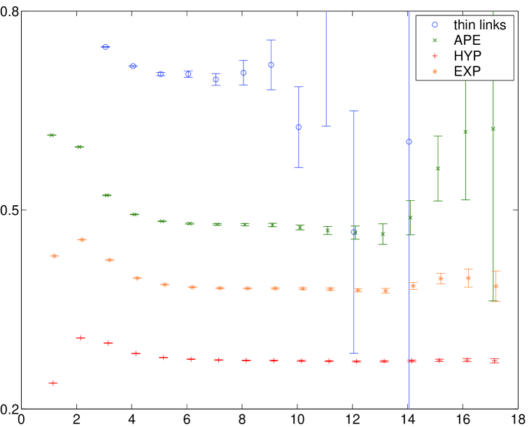
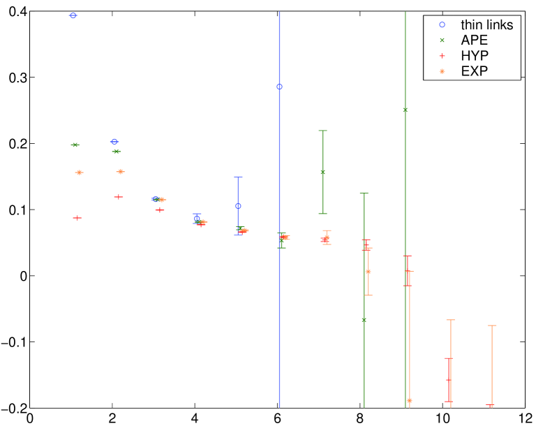
Figure 1: Top: $M_{\mathrm{eff}}(T)\!=\!{1\over 2}\log(W(R,T\!-\!1)/W(R,T\!+\!1))$ vs. $T$ at $R\!=\!3$ after one step with projection and $\alpha_{\mathrm{APE}}\!=\!0.5,\alpha_{\mathrm{HYP}}\!=\!(0.3,0.6,0.75),\alpha_{\mathrm{EXP}}\!=\!0.2$. The thick links at the initial and final time-slice result in a loss of overall positivity. For the relation of plateau-height and -length cf. Fig. 2. Bottom: $-\!\log(\chi(x))$ vs. $x$ without smearing and after one step as above. The data stem from $500$ configurations on a $12^{3}\!\times\!18$ lattice with the Wilson gauge action at $\beta\!=\!6.0$.

To test the hypothesis (21) it is useful to look at the symmetric diagonal Creutz ratio [17]

$$\chi(x) \equiv \sqrt{\chi_{+}(x,x)\chi_{-}(x,x)}$$ (22)

$$\chi_{+}(R,T) = {W(R,T)W(R\!+\!1,T\!+\!1)\over W(R\!+\!1,T)W(R,T\!+\!1)}\simeq e^{-\sigma}$$

$$\chi_{-}(R,T) = {W(R,T)W(R\!-\!1,T\!-\!1)\over W(R\!-\!1,T)W(R,T\!-\!1)}\simeq e^{-\sigma}$$

which (for large $x$) is independent of $\mu$. In Fig. 1 (bottom) $-\!\log(\chi(x))$ vs. $x$ is shown, both for the original loop and after one APE/HYP/EXP-step. The squared string tension is invariant under smearing, but the error-bar changes. HYP reduces it more aggressively than APE and EXP (for the parameters used in Fig. 1, the parameter dependence is addressed below).

In summary, Fig. 1 suggests that the reduced self energy of the quasi-static quark (i.e. its divergent piece $\delta m\!\sim\!1/a$) is responsible for the improved signal-to-noise ratio after smearing.

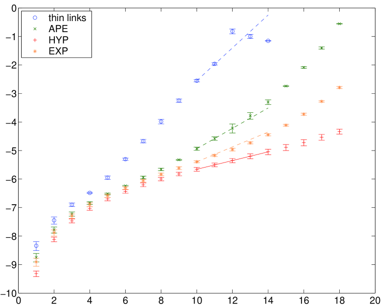
Figure 2: Log of noise over signal in the Wilson loop shown in Fig. 1 (top), without smearing and after one step of APE/HYP/EXP-smearing. The full line is a fit to the HYP-data with range $[10,14]$; the slopes of the dashed lines represent the prediction $(\ref{signaltonoise})$ based on the $\Delta E_{Q\overline{Q}}$ taken from Fig. 1 (top) at $T\!=\!7$. The error on the error is defined as as $((j_{2}\!-\!j_{4})^{2}+(j_{4}\!-\!j_{6})^{2})^{1/2}$ with $j_{n}$ the jackknife error at binlength $n$. Configurations and parameters are those of Fig. 1.

In fact, this discussion can be made more precise by virtue of an argument due to Lepage [16]. The key idea is rather than determining the variance of a correlator $C(x)=\langle O^{\dagger}(x)O(0)\rangle$ a posteriori from its fluctuation one could estimate it in the MC via $\langle O^{\dagger}(x)O(0)\tilde{O}^{\dagger}(0)\tilde{O}(x)\rangle$. Here, a different symbol has been chosen for the “copy” creation and annihilation operators to exclude additional unwanted Wick contractions, i.e. the idea is that they couple to different “flavors” (which, apart from the flavor number, have identical properties). In our case this noise-squared estimator consists of two Wilson loops, with opposite orientation, on top of each other. Asymptotically, it is dominated by two flux-tubes of length zero, i.e. by a state with mass $2V(0)\!=\!0$ for unitary links. Thus, since the original correlator falls of with an effective mass $E_{Q\overline{Q}}$ and its noise is asymptotically constant, the Lepage argument [16] predicts

$${\mathrm{signal}\over\mathrm{noise}}(t)\;=\;\mathrm{const}\;e^{-E_{Q\overline{Q}}\,t}$$ (23)

and Fig. 2 shows that this expectation is indeed well satisfied. It is clear that the specific recipes and parameters in Figs. 1,2 are irrelevant – the Lepage argument is a general one.

5 Matching boxes via the local force

Our goal is to compare various smearing recipes on lattices generated with either the Wilson gauge action or an improved one. In order to give a fair comparison, these lattices should be matched, i.e. have the same spacing $a$ in units of a physical scale. Ideally, this is done by computing the HQ potential, but rather than moving on to compute various $R\!\times\!T$ “thin-link” Wilson loops, I propose (specifically for the present investigation) two shortcuts.

The first one is to avoid the $T\!\to\!\infty$ extrapolation and to determine the force $F(R,T)\!=\!{1\over 2}(\partial_{R}\!+\!\partial_{R}^{*})M_{\mathrm{eff}}(R,T)$ with $M_{\mathrm{eff}}(R,T)\!=\!{1\over 2}\log(W(R,T\!-\!1)/W(R,T\!+\!1))$ at one fixed entry, and I choose $R\!=\!T\!=\!4$. Since there is no $T\!\to\!\infty$ extrapolation, one can stay in a relatively small volume and the finite-volume effect will be the same for all final (tuned) lattices.

The second shortcut is even less innocent. In order to get precise values for $F(4,4)$, one is tempted to use smeared links. From the observation of Ref. [3] that (one step of) smearing affects (for $R\!>\!2$) mainly the additive constant in the HQ potential, one expects $F(4,4)$ to be unchanged, since its arguments are large enough. This is indeed the plan; albeit with the proviso that all three smearing recipes will be used to have a cross check.

Hence, the problem with measuring only $F(4,4)$ is that the fixed time separation does not allow to select a definite state (ideally the groundstate), and the mixture of states that one has at $T\!=\!4$ may vary with the gauge action and the type of link used at $T\!=\!0$. Therefore, having several “thick” links as creation and absorption operators helps, since they couple differently to excited states and one may hope that the problem is detected, if it is numerically sizable.

		original	APE	HYP	EXP
W	$\beta\!=\!6.00$	0.0576 (60)	0.0550(10)	0.0513(06)	0.0550(07)
S	$\beta\!=\!4.40$	0.0692(115)	0.0594(21)	0.0555(13)	0.0589(16)
	$\beta\!=\!4.50$	0.0494 (75)	0.0462(15)	0.0452(09)	0.0474(11)
	$\beta\!=\!4.60$	0.0343 (51)	0.0388(10)	0.0376(07)	0.0398(07)
I	$\beta\!=\!2.65$	0.0557 (72)	0.0552(16)	0.0527(11)	0.0559(12)
	$\beta\!=\!2.75$	0.0396 (43)	0.0444(10)	0.0429(07)	0.0450(08)
	$\beta\!=\!2.85$	0.0371 (35)	0.0384(10)	0.0371(08)	0.0391(09)
DBW2	$\beta\!=\!1.01$	0.0605 (53)	0.0604(15)	0.0602(12)	0.0628(13)
	$\beta\!=\!1.04$	0.0466 (34)	0.0504(10)	0.0504(10)	0.0528(11)
	$\beta\!=\!1.07$	0.0469 (31)	0.0491(12)	0.0478(09)	0.0502(10)
BKL	$\beta\!=\!4.70$	0.0644(105)	0.0566(19)	0.0537(12)	0.0573(14)
	$\beta\!=\!4.75$	0.0384 (97)	0.0527(19)	0.0500(11)	0.0532(13)
	$\beta\!=\!4.80$	0.0645 (75)	0.0486(14)	0.0439(08)	0.0469(10)
L	$\beta\!=\!0.79$	0.0562 (63)	0.0551(17)	0.0541(11)	0.0562(12)
	$\beta\!=\!0.80$	0.0529 (53)	0.0505(13)	0.0490(09)	0.0512(10)
	$\beta\!=\!0.81$	0.0430 (48)	0.0482(12)	0.0477(08)	0.0502(09)

Table 3: Details of the tuning process to get approximately matched lattices. Given is the force $F(R,T)\!=\!{1\over 4}\log(W(R\!+\!1,T\!-\!1)/W(R\!+\!1,T\!+\!1)\!\cdot\!W(R\!-\!1,T\!+\!1)/W(R\!-\!1,T\!-\!1))$ on a $8^{4}$ lattice for $R\!=\!T\!=\!4$. The columns APE/HYP/EXP give the result after one step with the same parameters as in Fig. 1. The errors are from a jackknife with binlength 2, using 800 (W) or 200 (all other actions) configurations per run, after discarding 10 configurations for thermalization.

Table 3 gives details of the tuning process aimed at finding $\beta$-values which (approximately) match a quenched $\beta_{\mathrm{W}}\!=\!6.0$ with the Wilson gauge action. The sections “I” and “BKL” refer to the tree-level choice in (11, 12), i.e. $\tilde{c}_{1}\!=\!c_{1}$ and $\tilde{c}_{2}\!=\!c_{2}$ throughout.

	original	APE	HYP	EXP
S	4.459 (44)	4.427(30)	4.439(17)	4.429(22)
I	2.555(298)	2.632(42)	2.652(31)	2.643(37)
DBW2	0.999(276)	1.026(28)	1.047(14)	1.041(14)
BKL	—	4.720(13)	4.729(12)	4.726(12)
L	0.790 (14)	0.788(06)	0.796(06)	0.791(09)

Table 4: $\beta$-values needed with the Symanzik/Iwasaki/DBW2/Beinlich-Karsch-Laermann/ Langfeld actions to have an approximately matched lattice w.r.t. $\beta\!=\!6.0$ with the Wilson gauge action, from interpolating data of Table 3. The HYP-values will be used subsequently.

By linearly interpolating, for each action, the simulated couplings one finds the matched (according to the local force at $R\!=\!T\!=\!4$ criterion) $\beta$-values. Results are given in Table 4, without smearing in the first column (where the error is largest) and with one APE/HYP/EXP-step in subsequent columns. The unsmeared matched $\beta$-values are compatible with any smeared counterpart, but also the agreement among the smeared ones is satisfactory. We rate this as a sign that our interpolated matched couplings are essentially correct. Obviously, this does not invalidate the theoretical concerns discussed above, but apparently our statistical precision is not good enough to really suffer from this.

In [18] Necco gives an interpolation formula for $\log(r_{0}/a)$ versus $\beta$ for the Iwasaki- and the DBW2-action, analogous to the one in [19] for the Wilson gauge action. Solving them, one finds that a lattice with $\beta_{\mathrm{W}}\!=\!6.0$ is matched via $\beta_{\mathrm{I}}\!=\!2.635$ and $\beta_{\mathrm{DBW2}}\!=\!1.034$ when employing one of the RG-motivated actions, respectively. My $\beta_{\mathrm{I}}\!=\!2.652(31)$ and $\beta_{\mathrm{DBW2}}\!=\!1.047(14)$ are consistent. In spite of the limitations mentioned above one may thus feel confident that the $\beta$-values listed in Table 4 yield lattices which are reasonably (say: better than to 10%) matched.

6 Effect on square Wilson loops and the Creutz ratio

Whether an improved gauge action is worth the investment is usually decided on the basis of the cut-off effects involved. Another practically relevant criterion might be whether such an action is amenable to noise-reduction techniques like the APE/HYP/EXP-smearing discussed above. Obviously, physical observables should depend as little as possible on the details of the smearing process, e.g. the parameters employed.

Following Ref. [5], we shall first have a look at a few Wilson loops, comparing the effect of changing the parameter(s) and/or the iteration level.

To this end I have prepared 100 lattices of size $12^{4}$ for each gauge action, using the $\beta$-values of the HYP column in Table 4. After this is done, one applies the smearing recipes discussed in section 3, varying the parameters in a reasonable range. For HYP I choose to concentrate on the direction of the “canonical” $\alpha$-value introduced in [3], i.e. I consider six $\alpha$-values,

$$\begin{array}[]{ll}\mbox{APE}:&\alpha\in\{0.20,0.40,0.60,0.80,1.00,1.20\}\\ \mbox{HYP}:&\alpha\in\{0.25,0.50,0.75,1.00,1.25,1.50\}\cdot\alpha_{\mathrm{HYP}}^{\mathrm{std}}\quad\mbox{with}\;\;\alpha_{\mathrm{HYP}}^{\mathrm{std}}=(0.3,0.6,0.75)\\ \mbox{EXP}:&\alpha\in\{0.05,0.10,0.20,0.35,0.55,0.80\}\end{array}$$ (24)

where I deviate from Ref. [3] in my notation $\alpha_{\mathrm{HYP}}\!=\!(\alpha_{\mathrm{step\,1}},\alpha_{\mathrm{step\,2}},\alpha_{\mathrm{step\,3}})$. I choose to apply $2^{n}$ smoothing steps between successive measurements, resulting in the smearing levels

$$n_{\mathrm{tot}}\in\{1,3,7,15\}\;.$$ (25)

\psfrag{al_1}{$\alpha^{(1)}$}\psfrag{al_2}{$\alpha^{(2)}$}\psfrag{al_3}{$\alpha^{(3)}$}\psfrag{al_4}{$\alpha^{(4)}$}\psfrag{al_5}{$\alpha^{(5)}$}\psfrag{al_6}{$\alpha^{(6)}$}\includegraphics[width=239.00314pt,angle={0}]{figs_new/fig_smear_wil_lev1.eps}

\psfrag{al_1}{$\alpha^{(1)}$}\psfrag{al_2}{$\alpha^{(2)}$}\psfrag{al_3}{$\alpha^{(3)}$}\psfrag{al_4}{$\alpha^{(4)}$}\psfrag{al_5}{$\alpha^{(5)}$}\psfrag{al_6}{$\alpha^{(6)}$}\includegraphics[width=239.00314pt,angle={0}]{figs_new/fig_smear_sym_lev1.eps}

\psfrag{al_1}{$\alpha^{(1)}$}\psfrag{al_2}{$\alpha^{(2)}$}\psfrag{al_3}{$\alpha^{(3)}$}\psfrag{al_4}{$\alpha^{(4)}$}\psfrag{al_5}{$\alpha^{(5)}$}\psfrag{al_6}{$\alpha^{(6)}$}\includegraphics[width=239.00314pt,angle={0}]{figs_new/fig_smear_iwa_lev1.eps}

\psfrag{al_1}{$\alpha^{(1)}$}\psfrag{al_2}{$\alpha^{(2)}$}\psfrag{al_3}{$\alpha^{(3)}$}\psfrag{al_4}{$\alpha^{(4)}$}\psfrag{al_5}{$\alpha^{(5)}$}\psfrag{al_6}{$\alpha^{(6)}$}\includegraphics[width=239.00314pt,angle={0}]{figs_new/fig_smear_dbw_lev1.eps}

\psfrag{al_1}{$\alpha^{(1)}$}\psfrag{al_2}{$\alpha^{(2)}$}\psfrag{al_3}{$\alpha^{(3)}$}\psfrag{al_4}{$\alpha^{(4)}$}\psfrag{al_5}{$\alpha^{(5)}$}\psfrag{al_6}{$\alpha^{(6)}$}\includegraphics[width=239.00314pt,angle={0}]{figs_new/fig_smear_bkl_lev1.eps}

\psfrag{al_1}{$\alpha^{(1)}$}\psfrag{al_2}{$\alpha^{(2)}$}\psfrag{al_3}{$\alpha^{(3)}$}\psfrag{al_4}{$\alpha^{(4)}$}\psfrag{al_5}{$\alpha^{(5)}$}\psfrag{al_6}{$\alpha^{(6)}$}\includegraphics[width=239.00314pt,angle={0}]{figs_new/fig_smear_lan_lev1.eps}

Figure 3: For each gauge action $W_{1\times 1},W_{2\times 2},W_{4\times 4}$ is plotted versus the parameter number in (24), 0 indicates the unsmeared starting point. Throughout 1 smearing step (APE, HYP with projection) is applied. Best $W_{1\times 1}$-parameters are $\alpha_{\mathrm{APE}}\!\simeq\!0.7,\alpha_{\mathrm{HYP}}\!\simeq\!(0.3,0.6,0.75),\alpha_{\mathrm{EXP}}\!\simeq\!0.2$.

\psfrag{al_1}{$\alpha^{(1)}$}\psfrag{al_2}{$\alpha^{(2)}$}\psfrag{al_3}{$\alpha^{(3)}$}\psfrag{al_4}{$\alpha^{(4)}$}\psfrag{al_5}{$\alpha^{(5)}$}\psfrag{al_6}{$\alpha^{(6)}$}\includegraphics[width=239.00314pt,angle={0}]{figs_new/fig_smear_wil_lev3.eps}

\psfrag{al_1}{$\alpha^{(1)}$}\psfrag{al_2}{$\alpha^{(2)}$}\psfrag{al_3}{$\alpha^{(3)}$}\psfrag{al_4}{$\alpha^{(4)}$}\psfrag{al_5}{$\alpha^{(5)}$}\psfrag{al_6}{$\alpha^{(6)}$}\includegraphics[width=239.00314pt,angle={0}]{figs_new/fig_smear_sym_lev3.eps}

\psfrag{al_1}{$\alpha^{(1)}$}\psfrag{al_2}{$\alpha^{(2)}$}\psfrag{al_3}{$\alpha^{(3)}$}\psfrag{al_4}{$\alpha^{(4)}$}\psfrag{al_5}{$\alpha^{(5)}$}\psfrag{al_6}{$\alpha^{(6)}$}\includegraphics[width=239.00314pt,angle={0}]{figs_new/fig_smear_iwa_lev3.eps}

\psfrag{al_1}{$\alpha^{(1)}$}\psfrag{al_2}{$\alpha^{(2)}$}\psfrag{al_3}{$\alpha^{(3)}$}\psfrag{al_4}{$\alpha^{(4)}$}\psfrag{al_5}{$\alpha^{(5)}$}\psfrag{al_6}{$\alpha^{(6)}$}\includegraphics[width=239.00314pt,angle={0}]{figs_new/fig_smear_dbw_lev3.eps}

\psfrag{al_1}{$\alpha^{(1)}$}\psfrag{al_2}{$\alpha^{(2)}$}\psfrag{al_3}{$\alpha^{(3)}$}\psfrag{al_4}{$\alpha^{(4)}$}\psfrag{al_5}{$\alpha^{(5)}$}\psfrag{al_6}{$\alpha^{(6)}$}\includegraphics[width=239.00314pt,angle={0}]{figs_new/fig_smear_bkl_lev3.eps}

\psfrag{al_1}{$\alpha^{(1)}$}\psfrag{al_2}{$\alpha^{(2)}$}\psfrag{al_3}{$\alpha^{(3)}$}\psfrag{al_4}{$\alpha^{(4)}$}\psfrag{al_5}{$\alpha^{(5)}$}\psfrag{al_6}{$\alpha^{(6)}$}\includegraphics[width=239.00314pt,angle={0}]{figs_new/fig_smear_lan_lev3.eps}

Figure 4: For each gauge action $W_{1\times 1},W_{2\times 2},W_{4\times 4}$ is plotted versus the parameter number in (24), 0 indicates the unsmeared starting point. Throughout 7 smearing steps (APE, HYP with projection) are used. Best $W_{1\times 1}$-parameters are $\alpha_{\mathrm{APE}}\!\simeq\!0.6,\alpha_{\mathrm{HYP}}\!\simeq\!(0.3,0.6,0.75),\alpha_{\mathrm{EXP}}\!\simeq\!0.1$.

\psfrag{al_1}{$\alpha^{(1)}$}\psfrag{al_2}{$\alpha^{(2)}$}\psfrag{al_3}{$\alpha^{(3)}$}\psfrag{al_4}{$\alpha^{(4)}$}\psfrag{al_5}{$\alpha^{(5)}$}\psfrag{al_6}{$\alpha^{(6)}$}\includegraphics[width=239.00314pt,angle={0}]{figs_new/fig_smear_wil_lev5.eps}

\psfrag{al_1}{$\alpha^{(1)}$}\psfrag{al_2}{$\alpha^{(2)}$}\psfrag{al_3}{$\alpha^{(3)}$}\psfrag{al_4}{$\alpha^{(4)}$}\psfrag{al_5}{$\alpha^{(5)}$}\psfrag{al_6}{$\alpha^{(6)}$}\includegraphics[width=239.00314pt,angle={0}]{figs_new/fig_smear_wil_lev6.eps}

Figure 5: $W_{1\times 1},W_{2\times 2},W_{4\times 4}$ versus the smearing parameter in the APE and HYP procedure without projection, using 1 (left) or 3 (right) iterations, on Wilson backgrounds. Note the difference to the first graph in Fig. 3.

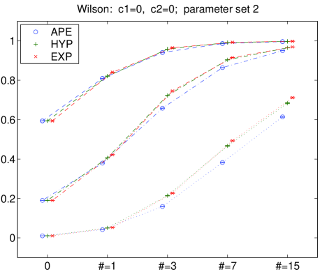
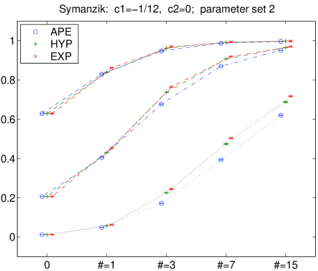
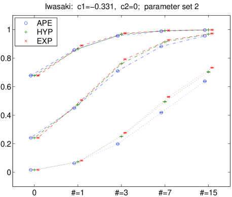
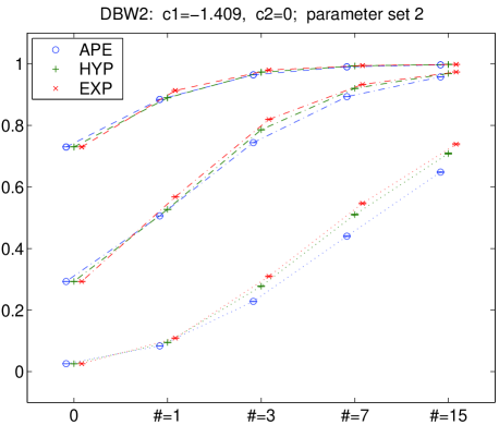
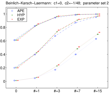
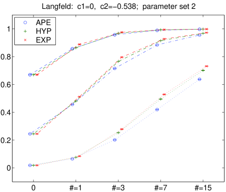
Figure 6: For each gauge action $W_{1\times 1},W_{2\times 2},W_{4\times 4}$ is plotted versus the number of smearing steps, 0 indicates the unsmeared starting point. Throughout the second parameter in (24) (APE, HYP with projection) is used: For small parameters many smearing steps seem favorable.

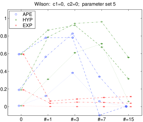
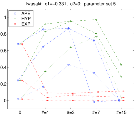
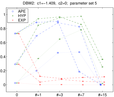
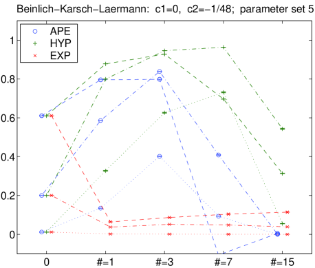
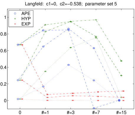
Figure 7: For each gauge action $W_{1\times 1},W_{2\times 2},W_{4\times 4}$ is plotted versus the number of smearing steps, 0 indicates the unsmeared starting point. Throughout the fifth parameter in (24) (APE, HYP with projection) is used: For large parameters the result deteriorates after a few steps.

Fig. 3 shows, for each action, the Wilson loops $W_{1\times 1},W_{2\times 2},W_{4\times 4}$ after 1 smearing step (with projection back to the gauge group) as a function of the smearing parameter. The plaquette gets increased for small $\alpha$ reaching a maximum around $\alpha_{\mathrm{APE}}\!\simeq\!0.7,\alpha_{\mathrm{HYP}}\!\simeq\!\alpha_{\mathrm{HYP}}^{\mathrm{std}},\alpha_{\mathrm{EXP}}\!\simeq\!0.2$; for larger parameters it decreases again. This holds for the larger Wilson loops, too, albeit the maximum may be shifted towards larger $\alpha$ (for APE and HYP). What all recipes have in common is that excessive parameters drive all loops to 0 (disorder) rather than to 1 (order).

Fig. 4 is the same after 7 smearing steps. For small $\alpha$ all Wilson loops are driven more efficiently to 1 than before, but beyond a certain “critical” parameter the descent to disorder is more pronounced, too. For APE and HYP this culminating $\alpha$ is barely changed compared to the previous figure, for EXP it is smaller.

Fig. 5 demonstrates a dramatic change in the behavior of any Wilson loop under smearing, if the projection in the APE or HYP recipe is abandoned. The graphs have been obtained with Wilson glue, but other actions yield the same type of monotonic decrease in $\alpha$.

Fig. 6 shows the Wilson loops $W_{1\times 1},W_{2\times 2},W_{4\times 4}$ (with projection in the APE and HYP cases) versus the iteration level for the second set of parameters in (24). With such small $\alpha$-values one always observes a benevolent pattern.

Fig. 7 shows that with somewhat larger parameters (throughout the fifth one out of the set (24)) iterating the smearing is not really a good idea. Note that these parameters are to the right of the maximum in Fig. 3, for “sub-critical” $\alpha$-values no such breakdown has been seen.

It is worth emphasizing how little the smearing “profile” depends on the gauge action, for matched ensembles. A maximum value of $P\!=\!\langle W_{1\times 1}\rangle$ might be used as a criterion to “optimize” the APE/HYP/EXP-parameters (the rather similar values with 1 and 7 iterations are found in the captions). Of course, such a criterion is arbitrary, but at least the result is universal, i.e. (to a good extent) independent of the gauge action used (for fixed physical spacing).

More interesting than the behavior of the Wilson loop itself is how the mean and the error of a physical observable derived from it evolve under smearing, i.e. whether different recipes yield consistent results. For that aim let us consider the squared string tension $\sigma\!=\!-\log(\chi)$ defined via the symmetric Creutz ratio (22), using the same gauge configurations as before.

\psfrag{al_1}{$\alpha^{(1)}$}\psfrag{al_2}{$\alpha^{(2)}$}\psfrag{al_3}{$\alpha^{(3)}$}\psfrag{al_4}{$\alpha^{(4)}$}\psfrag{al_5}{$\alpha^{(5)}$}\psfrag{al_6}{$\alpha^{(6)}$}\includegraphics[width=239.00314pt,angle={0}]{figs_new/fig_creutz_wil_lev2.eps}

\psfrag{al_1}{$\alpha^{(1)}$}\psfrag{al_2}{$\alpha^{(2)}$}\psfrag{al_3}{$\alpha^{(3)}$}\psfrag{al_4}{$\alpha^{(4)}$}\psfrag{al_5}{$\alpha^{(5)}$}\psfrag{al_6}{$\alpha^{(6)}$}\includegraphics[width=239.00314pt,angle={0}]{figs_new/fig_creutz_sym_lev2.eps}

\psfrag{al_1}{$\alpha^{(1)}$}\psfrag{al_2}{$\alpha^{(2)}$}\psfrag{al_3}{$\alpha^{(3)}$}\psfrag{al_4}{$\alpha^{(4)}$}\psfrag{al_5}{$\alpha^{(5)}$}\psfrag{al_6}{$\alpha^{(6)}$}\includegraphics[width=239.00314pt,angle={0}]{figs_new/fig_creutz_iwa_lev2.eps}

\psfrag{al_1}{$\alpha^{(1)}$}\psfrag{al_2}{$\alpha^{(2)}$}\psfrag{al_3}{$\alpha^{(3)}$}\psfrag{al_4}{$\alpha^{(4)}$}\psfrag{al_5}{$\alpha^{(5)}$}\psfrag{al_6}{$\alpha^{(6)}$}\includegraphics[width=239.00314pt,angle={0}]{figs_new/fig_creutz_dbw_lev2.eps}

\psfrag{al_1}{$\alpha^{(1)}$}\psfrag{al_2}{$\alpha^{(2)}$}\psfrag{al_3}{$\alpha^{(3)}$}\psfrag{al_4}{$\alpha^{(4)}$}\psfrag{al_5}{$\alpha^{(5)}$}\psfrag{al_6}{$\alpha^{(6)}$}\includegraphics[width=239.00314pt,angle={0}]{figs_new/fig_creutz_bkl_lev2.eps}

\psfrag{al_1}{$\alpha^{(1)}$}\psfrag{al_2}{$\alpha^{(2)}$}\psfrag{al_3}{$\alpha^{(3)}$}\psfrag{al_4}{$\alpha^{(4)}$}\psfrag{al_5}{$\alpha^{(5)}$}\psfrag{al_6}{$\alpha^{(6)}$}\includegraphics[width=239.00314pt,angle={0}]{figs_new/fig_creutz_lan_lev2.eps}

Figure 8: For each gauge action the squared string tension $\sigma\!=\!-\log(\chi(5))$ is plotted versus the parameter number in (24), 0 indicates the unsmeared starting point. Throughout 3 smearing steps have been applied. Data with negative central values have been removed.

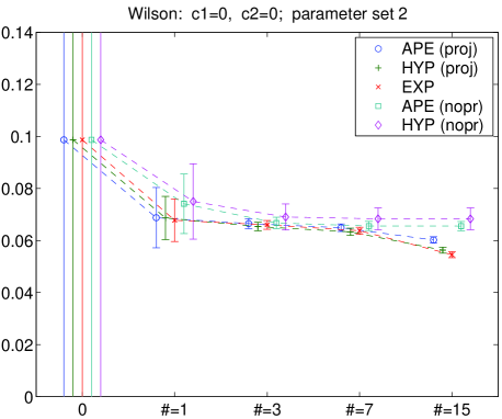
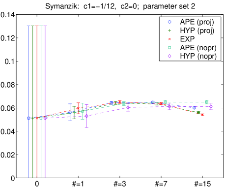
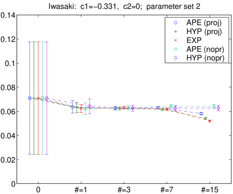
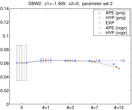
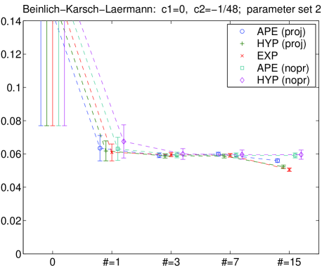
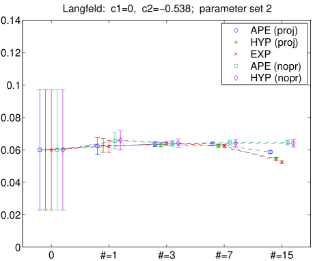
Figure 9: For each gauge action the squared string tension $\sigma\!=\!-\log(\chi(5))$ is plotted versus the number of smearing steps, 0 indicates the unsmeared starting point (where improved actions give a smaller error than the Wilson action). Throughout the second parameter in (24) is used.

Fig. 8 plots $-\log(\chi(5))$ versus the parameter $\alpha$ in (24) after 3 smearing steps. Moderate parameters suffice to tremendously reduce the noise and and different recipes prove consistent within errors. However, as the smearing parameter is raised beyond a reasonable level (typically something of the order of the “critical” parameter that achieved the maximum in the plaquette), the error may grow again. When repeating this with a higher iteration level basically the same behavior emerges, although the onset of systematic distortions with large parameters gets more pronounced. There are two more points that deserve a comment. First, I find it astonishing that the projection-free APE and HYP recipes manage to decrease the error in a physical observable, even though we have just seen that they drive the plaquette to 0 rather than 1. Does this indicate that the naive interpretation is wrong, and what one gets is not disorder but some type of anti-ferromagnetic ordering ? Obviously, this calls for further investigation, but it seems non-trivial to address this issue in a gauge-invariant manner without invoking extreme requests for CPU time. Finally, comparing the unsmeared values, one notices that all improved actions have an error bar which is smaller than the one with the Wilson action. Hence an improved action may lead to a smaller error (with identical statistics) in a gluonic observable, but it is clear that this is not competitive with the effect of smearing.

Fig. 9 plots $-\log(\chi(5))$ versus the number of smearing steps for the second parameter in the set (24). Here, a “plateau” includes $1$ to $\sim\!7$ iterations – further out consistency is lost. With a larger parameter a similar picture emerges, but the “plateau” ends earlier. Numerically, a value $\sigma\!\simeq\!0.06(1)$ corresponds to a string tension $\sqrt{\sigma}\!\simeq\!490(40)\,\mathrm{MeV}$, if $a^{-1}\!=\!2\,\mathrm{GeV}$ is assumed. Hence a statistical accuracy of 8% can be achieved with 100 lattices of size $12^{4}$.

In summary, these figures indicate a trade-off situation between a statistical error on one side and a systematic error on the other. Smearing reduces the former, but when applied in excess (either through too large a parameter or too many iterations) it introduces clear artifacts. It would be interesting to test how much of these can be attributed to the loss of locality. The good news is that a detailed optimization of the parameters is not needed – smearing proves beneficial as long as one can explicitly demonstrate that one is in the two-fold plateau; i.e. as long as a even larger parameters and/or higher iteration levels do not alter the result.

7 Effect on field-theoretic topological charge

Knowing that smearing reduces the UV-fluctuations and given the relation between UV-fluctuations and large renormalization factors and/or cut-off effects, one may ask whether smearing reduces the latter. An observable from which one can learn something in this respect without having to take the continuum limit is the “naive” field-theoretic topological charge

$$q_{\mathrm{nai}}[U]={1\over 4\pi^{2}}\int\!dx\;\mathrm{tr}(F_{12}F_{34}-F_{13}F_{24}+F_{14}F_{23})={1\over 32\pi^{2}}\int\!dx\;\mathrm{tr}(\epsilon_{\mu\nu\sigma\rho}F_{\mu\nu}F_{\sigma\rho})\;.$$ (26)

I have implemented (26) with $F_{\mu\nu}$ defined as the hermitean part of $-\mathrm{i}U_{\mu\nu}=-\mathrm{i}I+aF_{\mu\nu}+...$ where $U_{\mu\nu}(x)$ is the mean of the four plaquettes in the $(\mu,\nu)$-plane with starting point $x$. The goal is to see what happens if one replaces $U_{\mu\nu}$ by one which is constructed from smeared links.

Using the same 100 lattices (for each action) of size $12^{4}$ as in the previous section, I decided to stay with a single parameter fixed at near-optimal values (according to the $W(1,1)$ criterion), $\alpha_{\mathrm{APE}}\!=\!0.5$, $\alpha_{\mathrm{HYP}}\!=\!(0.3,0.6,0.75)$, $\alpha_{\mathrm{EXP}}\!=\!0.2$ and three smearing levels $n_{\mathrm{tot}}\in\{1,3,7\}$.

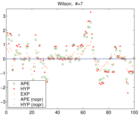
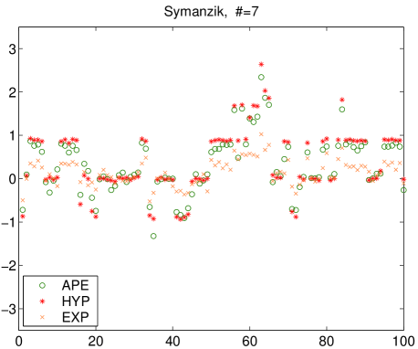
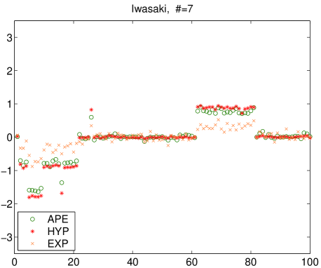
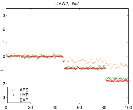
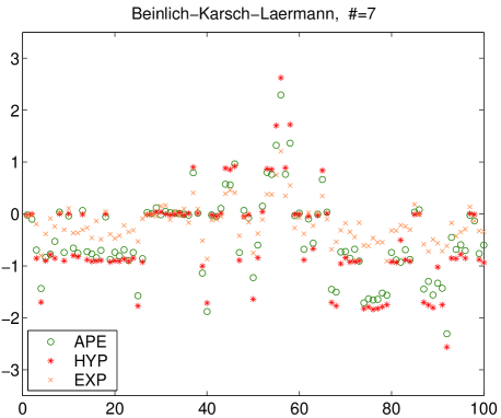
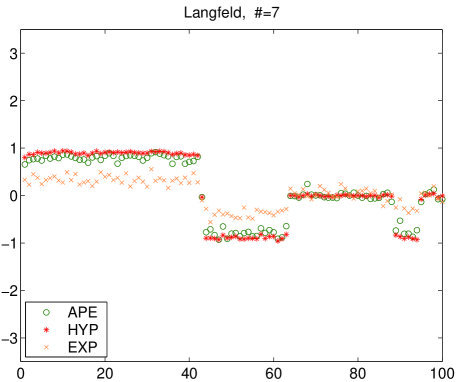
Figure 10: Time history of the bare topological charge (26) on the matched $12^{4}$ lattices after 7 smearing steps in the definition of $F_{\mu\nu}$ (parameters as in Fig. 11). The projection-free APE/ HYP-varieties always give a number very close to zero (omitted in the improved action panels).

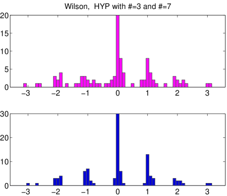
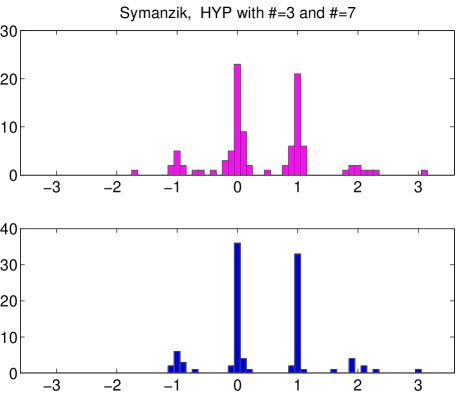
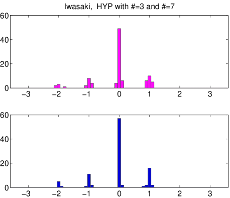
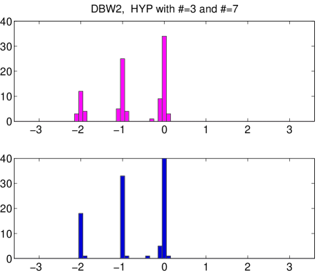
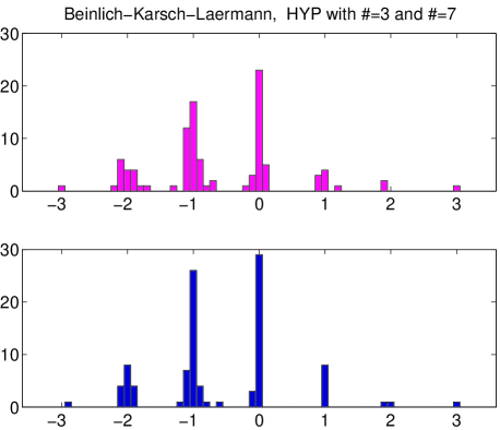
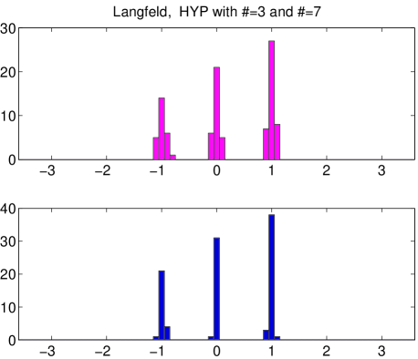
Figure 11: Histograms of the semi-renormalized topological charges after 3 (light) and 7 (dark) steps of HYP-smearing. The appropriate $Z$-factors have been applied, but not the “cast-to-integer” operation. The smearing parameter is $\alpha_{\mathrm{HYP}}\!=\!(0.3,0.6,0.75)$.

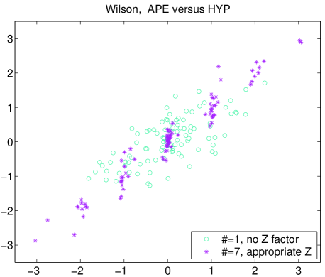
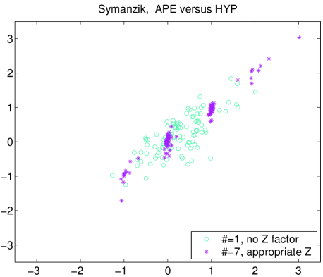
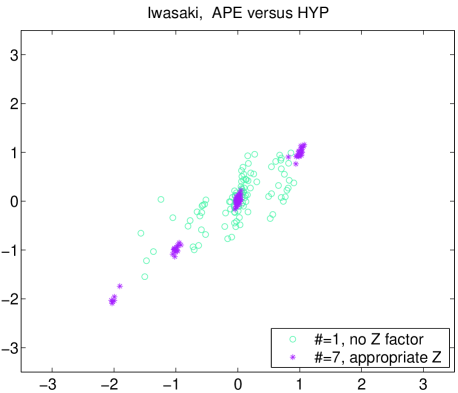
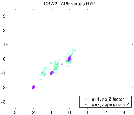
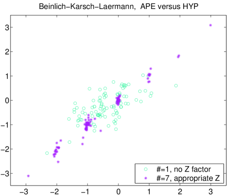
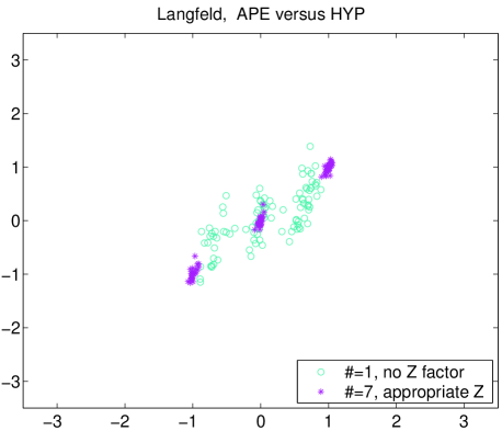
Figure 12: Correlation of the unrenormalized topological charges after 1 step of APE- or HYP-smearing $($light$)$ and of the semi-renormalized charges after 7 steps of APE- or HYP-smearing $($dark$)$. In the latter case, and with the final “cast-to-integer” operation performed, the number of configurations on which the APE- and HYP-charges disagree is $13,2,0,0,3,0$, respectively.

Fig. 10 shows the time evolution of the bare topological charge (26) after 7 smearing steps. The APE/HYP varieties without projection tend to drive $q_{\mathrm{nai}}[U]$ to zero for any gauge background; these symbols are shown only for the Wilson action. The results of all other recipes tend to cluster near non-integer values $n/Z$ with $n\!\in\!\mathbf{Z}$ and $Z$ a function of the smearing recipe (the order is $1\!<\!Z_{\mathrm{HYP}}\!<\!Z_{\mathrm{APE}}\!\ll\!Z_{\mathrm{EXP}}$ for our parameters, i.e. HYP and APE with projection require only moderate rescaling). This suggests a renormalization factor $Z$ such that $Zq[U]$ tends to cluster near integer values. Define – for a given smearing recipe and a given definition of $F_{\mu\nu}$ in (26) – the charge renormalization factor $Z$ as the solution of

$$\min_{Z>1}(\chi^{2})\quad\mathrm{where}\qquad\chi^{2}=\sum_{U}\Big{(}Z\,q_{\mathrm{nai}}[U]-\mathrm{nint}(Z\,q_{\mathrm{nai}}[U])\Big{)}^{2}\;.$$ (27)

Having $Z$ at hand, one may define the renormalized “naive” field-theoretic topological charge

$$q_{\mathrm{ren}}[U]=\mathrm{nint}(Z\,q_{\mathrm{nai}}[U])$$ (28)

which, by construction, is an integer. Employing such a definition one sees well-defined charge histories in each graph of Fig. 10. Obviously, we recover the standard wisdom that – at a fixed physical lattice spacing – the Wilson gauge action accomplishes topology changes more easily than the Symanzik, Iwasaki and DBW2 action (in this order). The same phenomenon happens for the $W^{2\times 2}$-actions; the larger $c_{2}$ the more difficult is it to tunnel into another sector.

Coming back to the definition (27, 28), the prime question is whether the assigned charge $q_{\mathrm{ren}}[U]$ is really a property of the gauge background $U$. Fig. 11 contains the histograms of $Zq$ after 3 and 7 HYP-steps ($Z$ depends both on the smearing level and the gauge action). Here, the valleys between the peaks are sufficiently depleted, and the cast-to-integer operation in (28) makes sense. Unfortunately, there is no real valley structure at the levels 0 and 1. Hence the question is to which extent such an integer-valued charge $q_{\mathrm{ren}}[U]$ is a genuine function of the background $U$ and to which extent it is an artifact of the smearing procedure.

The key to this issue is to compare different smearing recipes. Fig. 12 relates the unrenormalized APE- and HYP-charges after 1 and 7 smearing steps. In the former case there is some correlation between the unrenormalized $q_{\mathrm{nai}}[U]$, but there is no clustering whatsoever. In the latter case, i.e. after a few more smearing steps, the two rescaled $Zq_{\mathrm{nai}}$ cluster predominantly near the same integers. With 100 configurations in each ensemble, on 87/98/100/100/97/100 the 7-APE-step and 7-HYP-step charges agree after renormalization. Thus, for $a^{-1}\!\simeq\!2\,\mathrm{GeV}$ and an improved gauge action the two charges agree almost on a configuration-by-configuration basis and this suggests that such a charge is indeed a function of the background $U$.

Still, this does not mean that the renormalized “naive” field-theoretic charge (27, 28) is as much a clean concept as the fermionic charge defined through the index of the Dirac operator $q_{\mathrm{ind}}\!=\!{1\over 2}\mathrm{tr}(\gamma_{5}\,D)$ [20, 21] with $D$ any Dirac operator that satisfies the Ginsparg-Wilson relation [22]. However, (27, 28) has the virtue of being cheap in terms of CPU-time; the $O(3...7)$ smearing steps cost less than the hundreds of cooling steps that have been used in the past, and results are competitive with those of the cooling era (see e.g. Ref. [23] for a nice example). An issue that deserves further study is whether too much smearing eventually destroys the charge.

8 Summary

The goal of this work has been a comparison of the newly proposed EXP smearing [5] against the well established APE and HYP procedures [2, 3] on various gauge backgrounds.

I started by scanning through (part of) the space of parameters and iteration levels to see which combinations drive the plaquette and larger Wilson loops to 1 rather than 0 and to see whether the choice of the gauge action would have a big influence. The result is that standard parameters around $\alpha_{\mathrm{APE}}\!\simeq\!0.65,\alpha_{\mathrm{HYP}}\!\simeq\!(0.3,0.6,0.75),\alpha_{\mathrm{EXP}}\!\simeq\!0.15$ prove nearly optimal, at least if $O(1..3)$ iterations are performed. Obviously, the plaquette criterion is rather arbitrary, but for $a^{-1}\!\simeq\!2\,\mathrm{GeV}$ the result is universal, i.e. independent of the gauge action.

The only physics point of this paper has been an explicit test of the Lepage argument in the heavy-heavy case. This argument establishes a connection between the signal-to-noise ratio of an observable involving a static quark and the HQ self energy, and our Fig. 2 shows that it passed the test with flying colors. Hence a future optimization strategy tailored to HQ physics might be to reduce the HQ self energy as much as possible. The key insight is that in the case of large Wilson loops various smearing recipes differ in the signal generated, not in the noise.

Next I evaluated the squared string tension defined via the Creutz ratio at $R\!=\!T\!\simeq\!0.5\,\mathrm{fm}$. The main finding is that any smearing recipe drastically reduces the noise and a detailed tuning of parameters and/or iteration level is neither needed nor useful. Instead there is a broad two-dimensional plateau in which changing the two does not significantly alter the central value or the error. Only at absurdly high levels systematic effects get visible, presumably due to the reduced locality in terms of the original links. In summary, moderate smearing suggests itself as a simple and efficient means to damp the UV-noise in standard gluonic observables.

Finally, I have focused on the “naive” field-theoretic topological charge. Here, the power of any smearing recipe depends a lot on the gauge action used. The good news is that the lattice spacings where the smearing details implicit in the definition (26, 27, 28) prove irrelevant are accessible; for the Iwasaki action it is around $a\!\simeq\!0.1\,\mathrm{fm}$, for other actions not much below.

Acknowledgments: It is a pleasure to acknowledge useful correspondence with Silvia Necco as well as the benefits from a discussion with Rainer Sommer, Michele Della Morte and Francesco Knechtli on the Lepage argument. Computations were done on a PC at DESY Zeuthen. This work has been supported by the DFG in the framework SFB/TR-9.

Appendix: Projection details

Here I spell out the projection procedure introduced in [14]. For related ideas see [24, 25].

The idea is to define the projection step $V_{\mu}(x)\to W_{\mu}(x)$ via the overlap-type recipe

$$W_{\mu}(x)={V_{\mu}(x)\,[V_{\mu}(x)^{\dagger}V_{\mu}(x)]^{-1/2}\over[\det(\mathrm{numerator})]^{1/3}}$$ (29)

which leads to an eigenvector decomposition problem of the hermitean operator $X\!\equiv\!V^{\dagger}V$.

In principle, one might find the eigenvalues $x_{1},...,x_{3}$ of $X$ (following Cardano) by forming

$$a = -\mathrm{tr}(X)$$

$$b = X_{11}X_{22}+X_{22}X_{33}+X_{33}X_{11}-X_{12}X_{21}-X_{23}X_{32}-X_{31}X_{13}$$

$$c = -\det(X)$$

$$p = b-{a^{2}\over 3}$$

$$q = {2a^{3}\over 27}-{ab\over 3}+c$$

and continuing with

$$\mathrm{if}\;p=0\;\mathrm{then}\;u_{1}=\left\{\begin{array}[]{ll}0&\mathrm{if}\;q=0\\ ({1\over 2}+\mathrm{i}{\sqrt{3}\over 2})\sqrt[3]{q})&\mathrm{if}\;q>0\\ \sqrt[3]{-q}&\mathrm{if}\;q<0\end{array}\right\}\;\mathrm{and}\;\begin{array}[]{l}x_{1}=u_{1}-{a\over 3}\\ x_{2}=(-{1\over 2}+\mathrm{i}{\sqrt{3}\over 2})u_{1}-{a\over 3}\\ x_{3}=(-{1\over 2}-\mathrm{i}{\sqrt{3}\over 2})u_{1}-{a\over 3}\end{array}$$ (30)

$$\mathrm{else}\;\begin{array}[]{ll}u_{1}\!&\!=\;\sqrt[3]{-{q\over 2}+\sqrt[2]{{q^{2}\over 4}+{p^{3}\over 27}}}\\ v_{1}\!&\!=\;-{p\over 3u_{1}}\end{array}\;\;\mathrm{and}\;\;\begin{array}[]{l}x_{1}=u_{1}+v_{1}-{a\over 3}\\ x_{2}=(-{1\over 2}+\mathrm{i}{\sqrt{3}\over 2})u_{1}+(-{1\over 2}-\mathrm{i}{\sqrt{3}\over 2})v_{1}-{a\over 3}\\ x_{3}=(-{1\over 2}-\mathrm{i}{\sqrt{3}\over 2})u_{1}+(-{1\over 2}+\mathrm{i}{\sqrt{3}\over 2})v_{1}-{a\over 3}\end{array}$$ (31)

where the roots in (31) must be taken over the body of complex numbers, though the result $x_{1},...,x_{3}$ is real.

A practical problem emerges whenever $X$ is close to unity (what is generic after a few smearing iterations), as the naive implementation cannot separate the eigenvalues any more. In order to reduce numerical extinction, one should implement

$$Y={1\over 2}(V^{\dagger}\!-\!1)(V\!-\!1)+\mathrm{h.c.}+(V^{\dagger}\!-\!1)+(V\!-\!1)\qquad\Big{(}=X\!-\!1\Big{)}$$ (32)

rather than $X$ and trade, for the same reason, the quantities $a,b,c$ for alternative ones designed to involve only “small” numbers in the case $X\!\simeq\!1$:

$$a_{3}\! \!=\! \!-Y_{11}-Y_{22}-Y_{33}\qquad\Big{(}=a\!+\!3\simeq 0\Big{)}$$ (33)

$$b_{3} = Y_{11}Y_{22}+Y_{22}Y_{33}+Y_{33}Y_{11}-Y_{12}Y_{21}-Y_{23}Y_{32}-Y_{31}Y_{13}-2a_{3}\qquad\Big{(}=b\!-\!3\simeq 0\Big{)}$$ (34)

$$c_{1} = -Y_{11}Y_{22}Y_{33}-Y_{12}Y_{23}Y_{31}-Y_{32}Y_{21}Y_{13}$$ (35)

$$+Y_{11}Y_{23}Y_{32}+Y_{22}Y_{31}Y_{13}+Y_{33}Y_{12}Y_{21}-b_{3}-a_{3}\quad\Big{(}=c\!+\!1\simeq 0\Big{)}$$

$$p = b_{3}-{a_{3}^{2}\over 3}+2a_{3}$$ (36)

$$q = {2a_{3}^{3}\over 27}-{2a_{3}^{2}\over 3}+a_{3}-{a_{3}b_{3}\over 3}+b_{3}+c_{1}$$ (37)

before one proceeds with (30, 31), where again $y_{1}=u_{1}\;[+v_{1}]\,-{a_{3}\over 3}$, etc. should be formed rather than $x_{1},x_{2},x_{3}$. Knowing the eigenvalues (minus 1) with good precision, it is easy to find the eigenvectors of $X$ by solving the characteristic equation

$$Yv_{i}=y_{i}v_{i}\qquad(i\in\{1,..,3\})$$ (38)

and after normalizing them one forms

$$W={V\,\sum\limits_{i=1}^{3}v_{i}{1\over\sqrt{y_{i}+1}}v_{i}^{\dagger}\over[\det(\mathrm{numerator})]^{1/3}}\;.$$ (39)

Of course this costly projection procedure is only needed if the argument is potentially far away from $SU(3)$; whenever $V$ is known to be close to $SU(3)$ (e.g. in the MC a newly proposed link is projected to $SU(3)$ before it is subject to the accept/reject-test, but here the deviation is just due to round-off errors) one may project via an approximate procedure, e.g. via

$$V\;\longrightarrow\;V^{\prime}={3\over 2}V-{1\over 2}VV^{\dagger}V\;,\qquad V^{\prime}\;\longrightarrow\;V^{\prime\prime}=V^{\prime}\Big{(}1-{1\over 3}(\det V^{\prime}-1)\Big{)}\;.$$ (40)

Finally, it is worth mentioning that the same eigenmode decomposition technique (simplified by $a\!=\!0$) has been used in the matrix exponentiation in the EXP recipe (18).

References

• [1]
• [2] M. Albanese et al. [APE Collaboration], Phys. Lett. B 192, 163 (1987).
• [3] A. Hasenfratz and F. Knechtli, Phys. Rev. D 64, 034504 (2001) [hep-lat/0103029]. A. Hasenfratz, R. Hoffmann and F. Knechtli, Nucl. Phys. Proc. Suppl.  106, 418 (2002) [hep-lat/0110168].
• [4] K. Orginos, D. Toussaint and R.L. Sugar [MILC Collaboration], Phys. Rev. D 60, 054503 (1999) [hep-lat/9903032].
• [5] C. Morningstar and M.J. Peardon, Phys. Rev. D 69, 054501 (2004) [hep-lat/0311018].
• [6] T. Blum et al., Phys. Rev. D 55, 1133 (1997) [hep-lat/9609036].
• [7] K.G. Wilson, Phys. Rev. D 10, 2445 (1974).
• [8] K. Symanzik, Nucl. Phys. B 226, 187 (1983). K. Symanzik, Nucl. Phys. B 226, 205 (1983).
• [9] Y. Iwasaki, Tsukuba preprint, UTHEP-118, 1983.
• [10] P. de Forcrand et al. [QCD-TARO Collaboration], Nucl. Phys. B 577, 263 (2000) [hep-lat/9911033].
• [11] G.P. Lepage, L. Magnea, C. Nakhleh, U. Magnea and K. Hornbostel, Phys. Rev. D 46, 4052 (1992) [hep-lat/9205007]. C.J. Morningstar, Phys. Rev. D 48, 2265 (1993) [hep-lat/9301005]. B. Beinlich, F. Karsch and E. Laermann, Nucl. Phys. B 462, 415 (1996) [hep-lat/9510031].
• [12] K. Langfeld, hep-lat/0403018.
• [13] N. Cabibbo and E. Marinari, Phys. Lett. B 119, 387 (1982). A.D. Kennedy and B.J. Pendleton, Phys. Lett. B 156, 393 (1985).
• [14] J. Kiskis, R. Narayanan and H. Neuberger, Phys. Lett. B 574, 65 (2003) [hep-lat/0308033].
• [15] M. Della Morte, et al. [ALPHA Collaboration], Phys. Lett. B 581, 93 (2004) [hep-lat/0307021]. M. Della Morte, A. Shindler and R. Sommer, hep-lat/0506008.
• [16] G.P. Lepage, Nucl. Phys. Proc. Suppl.  26, 45 (1992).
• [17] M. Creutz, Phys. Rev. Lett.  45, 313 (1980). M. Creutz, “Quarks, Gluons and Lattices,” Cambridge University Press (1983), eqn. (19.2).
• [18] S. Necco, Nucl. Phys. B 683, 137 (2004) [hep-lat/0309017].
• [19] M. Guagnelli, R. Sommer and H. Wittig [ALPHA collaboration], Nucl. Phys. B 535, 389 (1998) [hep-lat/9806005].
• [20] P. Hasenfratz, V. Laliena and F. Niedermayer, Phys. Lett. B 427, 125 (1998) [hep-lat/9801021].
• [21] F. Niedermayer, Nucl. Phys. Proc. Suppl.  73, 105 (1999) [hep-lat/9810026].
• [22] P.H. Ginsparg and K.G. Wilson, Phys. Rev. D 25, 2649 (1982).
• [23] J. Grandy and G. Kilcup, Nucl. Phys. Proc. Suppl. 53, 560 (1997) [hep-lat/9609012].
• [24] C. Christou, A. Di Giacomo, H. Panagopoulos and E. Vicari, Phys. Rev. D 53, 2619 (1996) [hep-lat/9510023].
• [25] L. Giusti, C. Hoelbling and C. Rebbi, Nucl. Phys. Proc. Suppl.  83, 896 (2000) [hep-lat/9906004].
• [26] After this preprint has been posted, a proceedings contribution appeared with useful references to some of the algorithmic literature: P. de Forcrand and O. Jahn, hep-lat/0503041.