CERN-PH-TH/2004-169

Finite temperature phase transition
in the 4d compact U(1) lattice gauge theory

Michele Vettorazzo^a, and Philippe de Forcrand^a,b,

^aInstitute for Theoretical Physics, ETH Zürich, CH-8093 Zürich, Switzerland
^bCERN, Physics Dept., TH Unit, CH-1211 Geneva 23, Switzerland

Abstract
We study the phase diagram of the ${\rm 4d}$ compact ${\rm U(1)}$ gauge theory as a function of the number of Euclidean time slices. We use the helicity modulus [1] as order parameter to probe the phase transitions. The order of the transition along the phase boundaries is studied and the possibility of a continuum limit is discussed. We present new, strong evidence that the $T=0$ bulk phase transition is first-order.

1 Introduction

The way in which continuum QFT incorporates the definition of ‘temperature’ has many relations with the notion of dimensional reduction: one crucial ingredient is in fact the compactification of the temporal dimension, whose length is tuned as a free parameter according to

$$T=\frac{1}{\mid\hat{L}_{t}\mid}$$ (1)

where $T$ is the temperature and $\mid\hat{L}_{t}\mid$ is the (dimensionful) time extension. On the lattice Eq.(1) reads

$$T=\frac{1}{L_{t}a}$$ (2)

where $a$ is the lattice spacing and now $L_{t}$ is a pure integer number; in this case the notion of finite temperature requires the possibility of taking the limit $a\to 0$, and then to tune $L_{t}$ accordingly to keep $T$ fixed.

In this paper we consider the ${\rm 4d}$ compact ${\rm U(1)}$ gauge theory on a lattice at fixed $L_{t}$. We study its phase diagram and pay particular attention to the points at which a continuum limit might be extracted, namely the phase boundaries. This is an interesting generalization of the analogous problem at ‘zero temperature’ ($L_{t}=\infty$), still open from the theoretical point of view, where only recently convincing numerical evidence of the first order nature of the transition was obtained [1, 2]. Further investigations seem therefore well motivated.

The paper is organized as follows. In Sec. 2 we describe the model and fix the formalism. In Sec. 3 we introduce the definition of the order parameter and review some of its properties. In Sec. 4 we study the phase diagram of the model. Conclusions follow.

2 The model

We consider a four dimensional lattice $L_{s}^{3}\cdot L_{t}$ with periodic boundary conditions. We associate to each link $U_{\mu}(r)$ ($r=(x,y,z,t)$) connecting two neighboring sites an element of the group $U(1)$, namely $e^{i\theta_{\mu}(r)}$, where $\theta_{\mu}(r)=aeA_{\mu}(r)$ is proportional to the vector potential $A_{\mu}(r)$ and $e$ is the bare gauge coupling. The system is governed by the Wilson action

$$S=\beta\sum_{r,\mu<\nu}\cos(\theta_{P}(r))_{\mu\nu}$$ (3)

where $(\theta_{P}(x))_{\mu\nu}=\theta_{\mu}(x)+\theta_{\nu}(x+\hat{\mu})-\theta_{\mu}(x+\hat{\nu})-\theta_{\nu}(x)$ is the so-called plaquette angle, and $\beta=\frac{1}{e^{2}}$.

Figure 1: Cartoon of a temporal $(s,t)$ plaquette in the case $L_{t}=1$. The two spatial links cancel each other, leading to a decoupling of the temporal links.

The phase structure of this model is well known at zero temperature ($L_{t}=L_{s}=L$, $L\to\infty$): it has a strong coupling confining phase for $\beta<\beta_{c}$, and a weak coupling Coulomb phase for $\beta>\beta_{c}$. There is strong numerical evidence that the phase transition (at $\beta_{c}=1.0111331(15)$) is of first order [1][2] . Thus, in the extended phase diagram $(\beta,1/L_{t})$, we have a complete picture of the axis $1/L_{t}=0$.

There is another limiting case which is easy to understand, namely $L_{t}=1$: consider one temporal plaquette, represented in the cartoon of Fig. 1. In the case $L_{t}=1$ the temporal link is already a gauge invariant quantity, a Polyakov loop itself. Moreover, from Fig. 1 it is clear that around a temporal plaquette the two spatial links are actually the same link considered twice in opposite orientations, therefore they exactly cancel each other. The temporal plaquette angle is therefore

$$\theta_{s}(x)+\theta_{t}(x+\hat{s})-\theta_{s}(x)-\theta_{t}(x)=\theta_{t}(x+\hat{s})-\theta_{t}(x)$$ (4)

The contribution of the temporal plaquettes to the action is thus

$$S_{\rm temp.}=-\beta\sum_{P_{\rm temp.}}\cos\theta_{P}=-\beta\sum_{\vec{x}}\cos(\theta_{t}(\vec{x}+\hat{s})-\theta_{t}(\vec{x}))$$ (5)

and it is completely decoupled from the spatial plaquettes. Furthermore, Eq.(5) is the action of the ${\rm 3d}$ XY model. One then realizes that in the case $L_{t}=1$ the partition function of the model factorizes into

$$Z_{L_{t}=1}=Z_{\rm 3d\hskip 2.84544ptXY}\cdot Z_{\rm 3d\hskip 2.84544ptLGT}$$ (6)

namely we decompose the full partition function into that of the 3d XY model and that of the 3d $U(1)$ lattice gauge theory. We know that the former undergoes a phase transition of second order at $\beta=0.45420(2)$ [4], while the latter is always in the confined phase. We summarize the information gained so far about the phase diagram in Fig. 2.

Figure 2: Sketch of the phase diagram of the model, collecting the information about the two limiting situations $L_{t}=1$ and $L_{t}=\infty$.

In order to explore the phase structure of the model for a generic value of $L_{t}$ we need an order parameter; we introduce it in the next section.

3 The order parameter

To distinguish between confining and Coulomb behavior, we could monitor the expectation values of large Wilson loops, or the correlation of two Polyakov loops. However, we can also construct an observable which directly probes the large-distance properties of the system, and which has proven itself to be an efficient tool for analyzing a weak first-order transition [1]: the helicity modulus.

To introduce the helicity modulus for this theory, we first review the notion of response function to an external static field. Consider our four-dimensional lattice and choose an orientation $(\mu,\nu)$; if we call $L_{\rho},L_{\sigma}$ the two other (orthogonal) directions, a stack of $L_{\rho}\cdot L_{\sigma}$ parallel $(\mu,\nu)$ planes is thus defined. Let us modify the partition function of the system by imposing an external flux $\Phi$ through this orientation, as shown in Fig. 3; the flux is homogeneously spread over each of the parallel planes, meaning that $\Phi_{P}=\Phi/L_{\mu}L_{\nu}$ is assigned to each plaquette with orientation $(\mu,\nu)$, as written in the following equation

Figure 3: Graphical representation of the static external flux imposed through the $(\mu,\nu)$ orientation.

$$S(\Phi)=-\beta\sum_{P\in(\mu,\nu\hskip 2.84544pt{\rm orient.})}\cos(\theta_{P}+\frac{\Phi}{L_{\mu}L_{\nu}})-\beta\sum_{P\notin(\mu,\nu\hskip 2.84544pt{\rm orient.})}\cos\theta_{P}$$ (7)

One may wonder if this specific choice of spreading the external flux plays a role in our construction, but the answer is no, since in this Abelian theory a suitable change of variables [1] can vary at will the distribution of the flux, leaving the partition function of the system unchanged. Moreover, one can consider another point of view, and show that the external flux can actually be imposed also via a change of the boundary conditions from pure periodic to twisted: this is very easily accomplished if we impose, e.g., that each link $U_{\mu}(r)$ in a particular $\mu$ direction is identified with its image at distance $L_{\nu}$ up to a phase factor $e^{i\Phi/L_{\mu}}$:

$$\theta_{\mu}(x+L_{\nu})=\theta_{\mu}(x)+\frac{\Phi}{L_{\mu}}$$ (8)

Let us now consider the free energy of the system

$$F(\Phi)=-\log Z(\Phi)=-\log\int dUe^{-S(U;\Phi)}$$ (9)

and study its behavior in the two phases. In the confining phase the correlation length $\xi$ is finite (a natural scale in this phase is provided by the string tension $\sigma=1/\xi^{2}$), and the effect of the external flux, i.e., of the boundary conditions, decreases as $e^{-L_{\nu}/\xi}$. Therefore, in the thermodynamic limit, we obtain the result

$$F(\Phi)={\rm const.}\quad\forall\hskip 2.84544pt\Phi$$ (10)

The situation is different in the Coulomb phase, where the correlation length of the system is infinite (the Coulomb potential does not fix any scale in the system) and therefore the free energy of the system has a non-trivial dependence on $\Phi$. In order to understand quantitatively this dependence, consider Eq.(7) in the classical limit $\beta\to\infty$, where all fluctuations are suppressed and the action of Eq.(7) reduces to the following

$$S_{\rm classic}(\Phi)=-\beta\sum_{P\in(\mu,\nu\hskip 2.84544pt{\rm orient.})}\cos(\frac{\Phi}{L_{\mu}L_{\nu}})+{\rm const.}$$ (11)

namely, only the contribution of the twisted plaquettes is present. Consider the thermodynamic limit at finite temperature, i.e., keeping one size fixed and letting the others diverge. The product $L_{\mu}\cdot L_{\nu}$ diverges, whatever orientation we choose, therefore it is possible to expand Eq.(11) around its argument, and obtain

$$F_{\rm classic}(\Phi)-F_{\rm classic}(\Phi=0)=\frac{\beta}{2}\Phi^{2}\frac{L_{\rho}L_{\sigma}}{L_{\mu}L_{\nu}}$$ (12)

since the sum is over $V=L_{\mu}L_{\nu}L_{\rho}L_{\sigma}$ identical contributions. Some comments about this last equation are necessary: first of all, we showed in [1] that for a finite $\beta$, where fluctuations are present, Eq.(12) is only slightly modified, namely

$$F_{[{\rm finite}\hskip 2.84544pt\beta]}(\Phi)-F_{[{\rm finite}\hskip 2.84544pt\beta]}(\Phi=0)=\frac{\beta_{R}(\beta)}{2}\Phi^{2}\frac{L_{\rho}L_{\sigma}}{L_{\mu}L_{\nu}}$$ (13)

i.e. the bare coupling is replaced by a renormalized coupling, and this is all we need to effectively take into account the fluctuations of the system. Another remark is that Eq.(7) is $2\pi$ periodic in $\Phi$, while Eq.(13) is not. The corresponding modification of Eq.(13) is exponentially small in the flux $\Phi$ for small $\Phi$ [1], and plays no role in what follows.

Reconsider now Eq.(13), and define

$$h(\beta)=\frac{\partial^{2}F(\Phi)}{\partial\Phi}\mid_{\Phi=0}$$ (14)

This quantity is called helicity modulus in the literature, and it is a measure of the curvature of the free energy profile around $\Phi=0$. From our previous discussion about the behavior of $F(\Phi)$ in the two phases, it follows that $h(\beta)$ is an order parameter for our theory. If one performs explicitly the double derivative w.r.t. $\Phi$, one finds

$$h(\beta)=\frac{1}{(L_{\mu}L_{\nu})^{2}}\{\langle\sum_{P\in(\mu,\nu\hskip 2.84544pt{\rm orient.})}\beta\cos\theta_{P}\rangle-\langle(\sum_{P\in(\mu,\nu\hskip 2.84544pt{\rm orient.})}\beta\sin\theta_{P})^{2}\rangle\}$$ (15)

directly amenable to numerical simulations.

It is important to observe that in our finite temperature system we expect a different response of the system to fluxes imposed through spatial or temporal orientation. Consequently the helicity modulus is expected to show different behavior. In the following we will carefully distinguish the two situations, calling spatial (resp. temporal) helicity modulus the response to a flux through spatial (resp. temporal) planes.

4 Phase structure of the model

Figure 4: Conjectured phase diagram of the model. The phase boundary on the left separates a confining phase from a partially Coulomb phase, in which static electric charges propagating in the temporal direction interact Coulombically while magnetic charges propagating in a spatial direction are confined. The phase boundary on the right separates this partially Coulomb phase from a pure Coulomb phase. The dotted line indicates the possibility that the transition remain second order for a range $1\leq L_{t}\leq\bar{L}_{t}$ of temporal sizes.

Let us go back to Fig. 2 and try to make an educated guess about the phase structure of the model. First of all, we expect a phase boundary connecting the first order transition point at $L_{t}=\infty$ with the second order point at $L_{t}=1$ (see Fig. 4). On the left of this curve we are in a confining phase; on the right we expect a different behavior of temporal and spatial helicity moduli. A natural possibility is that the $T=0$ transition between the confined and Coulomb phases splits for the two orientations at finite temperature. As a consequence we would have an intermediate phase in which temporal Wilson loops obey perimeter law, while spatial ones would still show confinement (area law), just like in the high temperature phase of Yang-Mills theories.

Another important issue is the order of the phase transition along the phase boundary on the left: we know that in the two limiting cases ($L_{t}=1$ and $L_{t}=\infty$) the order of the transition is different. Two scenarios are possible: either the transition remains more and more weakly first order, and turns to second order only when $L_{t}=1$, or there is some special value $\bar{L}_{t}>1$ for which the transition turns already to second order. This second scenario is represented in Fig. 4 by the dashed line.

Let us now consider and analyze separately the two conjectured phase boundaries, to understand the structure of the model as the thermodynamic limit is approached.

4.1 Transition to the Coulomb phase

In this section we consider the phase boundary on the right in Fig. 4, the one connecting the temporal Coulomb phase with the pure Coulomb phase. To explore this transition we want to observe a change of behavior (from area to perimeter law) in the spatial loops, therefore we have to probe the response of the system to external fluxes through spatial planes. Equivalently, we will consider the spatial helicity modulus.

In Fig. 5 we show the numerical results for the spatial helicity modulus, measured on a set of lattices with temporal size $L_{t}=2$ and different spatial sizes $L_{s}$. What is apparent is that the transition point does not seem to converge at all to some fixed value $\beta_{c}$, but moves to higher and higher values with the spatial lattice size. If this is the case, this transition disappears from the phase diagram in the thermodynamic limit.

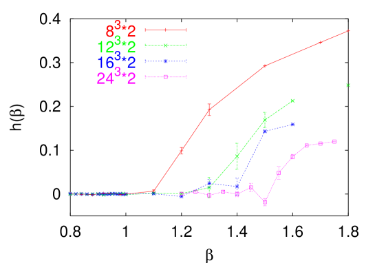
Figure 5: Spatial helicity modulus as a function of $\beta$, measured for a temporal size $L_{t}=2$ and for different $L_{s}$. The value of $\beta$ at the apparent transition point grows with the spatial size $L_{s}$. In the thermodynamic limit this phase boundary disappears.

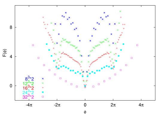
Figure 6: Flux free energy for lattices with temporal size $L_{t}=2$ and increasing spatial size, at $\beta=1.4$. As $L_{s}\to\infty$ the flux free energy tends to zero, as expected from Eq.(16).

A first rough way to understand the behavior of the system in this case is given by Eq.(13). Let us rewrite it here, focusing our attention on the geometrical factor

$$F_{[{\rm finite}\hskip 2.84544pt\beta]}(\Phi)-F_{[{\rm finite}\hskip 2.84544pt\beta]}(\Phi=0)=\frac{\beta_{R}(\beta)}{2}\Phi^{2}\frac{L_{s}L_{t}}{L_{s}L_{s}}$$ (16)

where we have highlighted the role of the spatial and temporal directions in this case. At any fixed value of $\Phi$ and at any finite $\beta$ we get therefore

$$F(\Phi)-F(0)\sim\frac{\beta_{R}}{L_{s}}\to 0\hskip 7.11317pt{\rm as}\hskip 7.11317ptL_{s}\to\infty$$ (17)

meaning that the flux free energy always vanishes in the thermodynamic limit; this prediction is nicely confirmed in Fig. 6, where $F(\Phi)$ is measured from the flux distribution $\nu(\Phi)=e^{-F(\Phi)}$ for different spatial extensions $L_{s}$. As a consequence, no phase transition is present between the mentioned phases for any finite value of $L_{t}$, but just the interplay of the coupling and of the spatial lattice size mimics a transition.

An alternative way to understand this finite size effect is the following. At any given value of $\beta$ there is a finite density of magnetic monopole currents. In particular, a wrapping (non-contractible) time-like current loop, far apart from its companion anti-loop, can disorder all the spatial planes in the lattice, or, equivalently, a spatial Wilson loop of arbitrary size; this, in turn, produces confinement [1]. Call $\rho(\beta)$ the density of currents at a given value of $\beta$; we know [5] that

$$\rho(\beta)\sim e^{-c\beta}$$ (18)

where $c$ is a constant, for $\beta\gg 1$. Let $n(l)dl$ be the distribution function indicating the fraction of monopole loops of length between $l$ and $l+dl$. The transition occurs approximately when each configuration contains a pair of non-contractible monopole loops, namely when

$$\rho(\beta)L_{s}^{3}\int_{l\geq 2L_{t}}n(l)dl\gtrsim 1$$ (19)

where the integration domain $l\geq 2L_{t}$ represents at least a necessary condition to have wrapping loops; on average we expect it to be also sufficient. The last piece of information we need is

$$\frac{dn(l)}{dl}\sim e^{-\delta l}$$ (20)

motivated by the fact that the free energy cost of a current is proportional to its length $l$ (notice that this is true only in the Coulomb phase, where the coefficient $\delta>0$). Let us put together all the ingredients and rewrite Eq.(19)

$$L_{s}^{3}e^{-c\beta}\int_{2L_{t}}^{\infty}e^{-\delta l}dl=L_{s}^{3}e^{-c\beta}\frac{e^{-2\delta L_{t}}}{\delta}\gtrsim 1$$ (21)

which contains all the information we need. At fixed volume, the inequality is satisfied only for sufficiently low $\beta$; when $\beta$ is large enough we are always in an ordered phase, as indicated by our numerical finding (spatial helicity modulus different from zero). In the limit $L_{s}\to\infty$ at fixed $L_{t}$, this equation is always satisfied, indicating that the system is always disordered. It is only in the limit $L_{t}\to\infty$ (because of the term $e^{-2\delta L_{t}}$) that we can obtain an ordered phase. Interestingly, this equation predicts a pseudocritical coupling

$$\beta_{c}\sim\log L_{s}$$ (22)

contrary to the simpler argument in Eq.(17) which gives

$$\beta_{c}\sim L_{s}$$ (23)

The first argument is completely classical, therefore we expect that Eq.(22) describes the physics better.

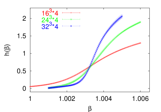
Figure 7: Temporal helicity modulus as a function of $\beta$, measured on systems of temporal size $L_{t}=4$ and different spatial sizes $L_{s}$.

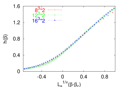
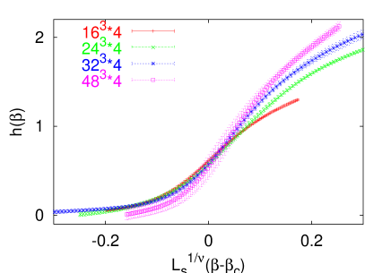
Figure 8: Finite-size scaling analysis of the temporal helicity modulus for lattices of temporal extent $L_{t}=2$ (left) and $L_{t}=4$ (right). The scaling window becomes narrower as $L_{t}$ increases, consistent with the approach to a first order transition.

4.2 Transition to the confining phase

Let us now turn our attention to the left phase boundary in Fig. 4, and to the temporal helicity modulus. Eq.(13) gives

$$F_{[{\rm finite}\hskip 2.84544pt\beta]}(\Phi)-F_{[{\rm finite}\hskip 2.84544pt\beta]}(\Phi=0)=\frac{\beta_{R}(\beta)}{2}\Phi^{2}\frac{L_{s}L_{s}}{L_{s}L_{t}}\sim L_{s}\beta_{R}(\beta)$$ (24)

therefore in the thermodynamic limit, at the transition point, the signal is infinitely enhanced; the transition point is determined (up to finite size effects) by the behavior of $\beta_{R}(\beta)$, which is related to the free energy of a monopole current, an order parameter by itself. In Fig. 7 we show one set of results for $L_{t}=4$ and three spatial volumes (the data are reweighted $\grave{a}$ la Ferrenberg-Swendsen [6]). From a finite size scaling analysis of such data we can extract the numerical value of $\beta_{c}$ as a function of the time extension $L_{t}$, and the order of the transition. For small values of $L_{t}$ we want to decide if the transition is first or second order. Our strategy is to assume the second order scenario (the universality class is then that of the ${\rm 3d~{}XY}$ model, as for $L_{t}=1$) and then check the quality of the data collapse. We thus fix $\nu=0.6723$ (the value of the ${\rm 3d}$ XY model [3]) and rescale the $\beta$ axis according to

$$\beta\to L_{s}^{1/\nu}(\beta-\beta_{c})\sim(\frac{L_{s}}{\xi})^{1/\nu}$$ (25)

where we have to tune $\beta_{c}$ only. The results of such analysis for the lattices with $L_{t}=2,4$ are presented in Fig. 8. Comparing the excellent collapse of the curves in the case $L_{t}=2$ with the mediocre collapse in the case $L_{t}=4$, one gets a first qualitative indication of a second order transition turning into a first order one. Moreover, one can speculate that for small values of $L_{t}>1$ the transition still is second order, as indicated in the cartoon of the phase diagram of Fig. 4. Since this issue is relevant to the possibility of extracting a continuum limit, we further investigated this problem directly by measuring the latent heat of the transition as a function of $L_{t}$. We took the direct approach of monitoring the Monte-Carlo history of the plaquette, starting from hot and cold (disordered and ordered) initial configurations. When a metastability is observed, we measure the distance between the two plateau values. We repeated the measurements for different volumes in order to keep the finite volumes effects under control. The plaquette histories are displayed in Fig. 9, and the estimated latent heats $\Delta E(L_{t})$ in Fig. 10. Table I summarizes our measurements of the critical parameters. As far as we know there are no theoretical predictions about the functional form that we observe for $\Delta E(L_{t})$. The data anyway seem to suggest a scenario in which the latent heat drops to zero already for $\bar{L}_{t}\sim 4$, at $\beta_{c}(L_{t})\sim 1$.

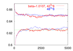
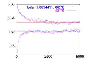
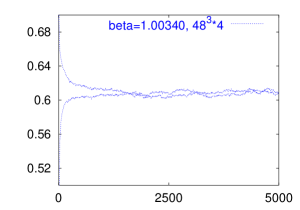
Figure 9: Time history of the plaquette, starting from an ordered (upper curves) and disordered (lower curves) initial state. The latent heat is defined as the difference of the values of the two plateaus. From left to right the cases $L_{t}=8,6,4$ are studied. For $L_{t}=8,6$, where the latent heat is certainly different from zero, we checked that the thermodynamic limit had been reached by comparing different spatial volumes.

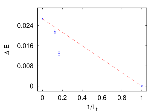
Figure 10: Latent heat $\Delta E$ of the transition versus $1/L_{t}$. The displayed data correspond to $L_{t}=\infty$, then $L_{t}=8,6,1$. The cases $L_{t}=4$ and $2$ are not displayed because the question whether the latent heat is already zero cannot be resolved with our numerical measurements. The dashed line corresponds to the simplest, linear ansatz.

$L_{t}$	$\Delta E$	$\beta_{c}$
$\infty$	0.02672(6) [2]	1.011331(15) [2]
8	0.0216(7)	1.0107(1)
6	0.0129(9)	1.009449(1)
4	-	1.00340(1)
3	-	0.989(1)
2	-	0.9008(3)
1	0	0.45420(2) [4]

Table 1: Latent heat $\Delta E$ and transition coupling $\beta_{c}$ versus $L_{t}$. $\Delta E$ decreases very quickly for $L_{t}<6$, opening the possibility of a second order phase transition for $L_{t}\lesssim 4$.

We cannot exclude a small but non-zero latent heat of course. However, Eq.(24) suggests that the transition turns from first- to second-order when $\beta_{R}(\beta_{c})$ vanishes as the transition point $\beta_{c}$ is approached from above, since then the magnitude of the jump in the helicity modulus at the phase transition also vanishes. The rapid decrease of $\beta_{R}$ with $\beta$ observed at zero temperature in [1] makes it unlikely that $\beta_{R}$ would remain non-zero all the way down to $\beta_{c}(L_{t}=1)\approx 0.45420$. Thus, we consider the scenario where the transition is second-order for a range of temporal sizes $[1,\bar{L}_{t}]$ as a likely alternative.

This opens the intriguing possibility of a continuum limit, obtained by approaching any point along such a second-order line. Note however that the number $L_{t}$ of time-slices cannot exceed $\bar{L}_{t}$, so that one cannot strictly speaking talk about the $U(1)$ system being at “finite temperature”. Rather, we have a system of $L_{t}\leq\bar{L}_{t}$ coupled ${\rm 3d-}$systems. Moreover, as one approaches the critical point, only the temporal correlation length $\xi_{t}/a$ diverges in lattice units, whereas the spatial correlation length $\xi_{s}/a$ remains finite. Thus, keeping the “physical” correlation length $\xi_{t}$ constant would imply not only $a\to 0$, but also $\xi_{s}\to 0$, so that the spatial planes would be completely disordered. The physical relevance of this situation seems marginal.

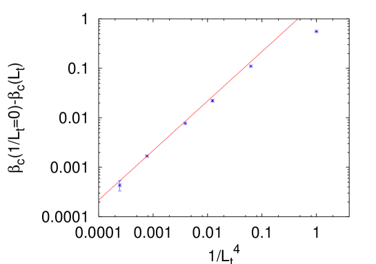
Figure 11: Shift of $\beta_{c}$ as a function of the Euclidean time extent $L_{t}$. The scaling ansatz shown is $\frac{c}{L_{t}^{1/\nu}}$, with $c=2.18$ and $\nu=1/4$. An exponent $\nu=1/d$ is the typical signature of a first-order phase transition.

The data in Table I can also be used for another kind of analysis, namely to study the dependence of $\beta_{c}$ on $L_{t}$ as $L_{t}\to\infty$. The coupling at the transition should in fact approach its asymptotic value $\beta_{c}(1/L_{t}=0)$ with typical finite-size corrections:

$$\beta_{c}(L_{t})\approx\beta_{c}(1/L_{t}=0)+\frac{c}{L_{t}^{1/\nu}}$$ (26)

where $c$ is a constant, and $\nu=\frac{1}{d}=\frac{1}{4}$ for a first-order transition. This is indeed the case, as shown in Fig. 11, where the straight line corresponds to $1/L_{t}^{4}$ corrections. This represents a qualitatively new and strong evidence of the first order nature of the transition in the zero temperature limit.

5 Conclusions

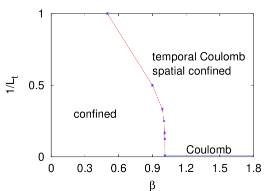
Figure 12: Phase diagram of the model. The phase boundary is obtained from a finite-size scaling analysis of the temporal helicity modulus. Three phases are indicated: a confining phase on the left of the phase boundary, a temporal Coulomb phase on the right of the boundary at finite $L_{t}$, and the pure Coulomb phase on the right of the boundary and for $L_{t}=\infty$.

In this paper we have investigated the phase diagram of the $4d$ $U(1)$ lattice gauge theory in the extended plane $(\beta,1/L_{t})$, where $L_{t}$ is the number of time-slices of the system. A summary of our findings is provided by Fig. 12 where the phase diagram of the model is shown. Only one phase boundary is present, whose position we have determined. It divides a confining phase on the left and a temporal Coulomb phase (with broken global $U(1)$ symmetry) on the right for any finite $L_{t}$; the pure Coulomb phase exists only for $L_{t}=\infty$ and $\beta>\beta_{c}=1.0111331(15)$. This phase diagram is remarkably similar to what we find in Yang-Mills theories, where spatial confinement persists at all temperatures.

The order parameter we used, the helicity modulus, reduces naturally, via dimensional reduction, to the ordinary helicity modulus known in condensed matter. We can therefore say that our order parameter is a generalization for gauge theories of the already known quantity.

The transition for any finite value of $L_{t}$ is first order, except perhaps for $L_{t}\lesssim 4$. In this case the transition becomes so weak that we cannot determine its order, but consider likely the possibility of a second order phase transition. This question could be studied by more powerful numerical methods. For instance, one could implement spatial $C$-periodic boundary conditions, which reduce the global $U(1)$ symmetry to $Z_{2}$, then measure the height of the free energy barrier between the two vacua as a function of the system size.

However, even if the transition is confirmed to be second order for $L_{t}\lesssim 4$, the relevance of this result to a continuum limit of the finite temperature $U(1)$ theory is marginal: in order to introduce the notion of temperature

$$T=\frac{1}{L_{t}a}$$ (27)

one must tune $L_{t}$ as a function of $a\to 0$ in order to maintain a finite $T$. If, as in our case, $L_{t}$ cannot be larger than a certain $\bar{L}_{t}$, the continuum limit cannot be taken, and we should not really talk about “finite temperature”.

Finally, we would like to mention the old paper [7], where the authors considered the Georgi-Glashow model with gauge group $SU(2)$ at finite temperature; this model reduces to our $U(1)$ model in the limit of complete gauge symmetry breaking (where $U(1)$ is the symmetry remnant of the broken $SU(2)$). The conjecture of the authors about the phase diagram of our model, contained in their Fig. $1$, is completely consistent with our findings.

An even older, correct, phase diagram can be found in [8]. The persistence of the spatial area law at finite temperature was first proven in [9].

6 Acknowledgement

We gratefully acknowledge Jürg Fröhlich, Oliver Jahn and Ben Svetitsky for useful discussions.

References

- [1] M. Vettorazzo and P. de Forcrand, Nucl. Phys. B 686, 85 (2004) [arXiv:hep-lat/0311006].
- [2] G. Arnold, B. Bunk, T. Lippert and K. Schilling, Nucl. Phys. Proc. Suppl. 119, 864 (2003) [arXiv:hep-lat/0210010].
- [3] M. Hasenbusch and T. Torok, arXiv:cond-mat/9904408.
- [4] A. P. Gottlob and M. Hasenbusch, PhysicaA 201, 593 (1993).
- [5] T. A. DeGrand and D. Toussaint, Phys. Rev. D 22, 2478 (1980).
- [6] A. M. Ferrenberg and R. H. Swendsen, Phys. Rev. Lett. 61(1988) 2635.
- [7] A. S. Kronfeld, M. L. Laursen, G. Schierholz and U. J. Wiese, Phys. Lett. B 198, 516 (1987).
- [8] B. Svetitsky, Phys. Rept. 132 (1986) 1.
- [9] C. Borgs, Nucl. Phys. B 261 (1985) 455.