Hadronic physics with domain-wall valence and improved staggered sea quarks

Abstract

With the advent of chiral fermion formulations, the simulation of light valence quarks has finally become realistic for numerical simulations of lattice QCD. The simulation of light dynamical quarks, however, remains one of the major challenges and is still an obstacle to realistic simulations. We attempt to meet this challenge using a hybrid combination of Asqtad sea quarks and domain-wall valence quarks. Initial results for the proton form factor and the nucleon axial coupling are presented.

1 INTRODUCTION

The simulation of light dynamical quarks constitutes one of the major challenges in contemporary lattice gauge theory research. The computational obstacle has in the past been addressed by investigating new algorithms, see, e.g. [1] and references therein.

Recently, a new approach has been attempted employing a so-called “hybrid” scheme where different types of sea and valence quarks are used, see [2]. It turned out that this calculation is extremely successful in predicting spectroscopic mass splitting in heavy quark physics correctly.

In this work we employ another type of hybrid calculation involving improved Kogut-Susskind sea quarks (Asqtad action [3]) and domain-wall valence fermions [4]. This scheme — although breaking unitarity at finite lattice spacing — will still have the same continuum limit as a fully dynamical calculation provided this limit exists. The quark masses of sea and valence quarks have to be properly tuned. The quantities we investigate are special cases of generalized parton distributions (GPDs) [5]. These have both parton distributions and form factors as certain limits and have already been studied on the lattice using conventional schemes [6].

This presentation is organized as follows: After discussing the tuning of the parameters of the valence domain-wall action in Section 2, we present the main results in Section 3. Finally, we summarize our findings and give an outlook for our ongoing research in Section 4.

2 CHOICE OF PARAMETERS

The two essential parameters we have to set are the size of the fifth dimension, $L_{5}$, for the domain-wall fermions and the bare quark mass parameter, $(am)_{q}^{\mbox{\tiny DWF}}$. The tuning of these two parameters is discussed in this section. The resulting parameters and sample sizes are summarized in Table 1.

Table 1: Parameters of our runs after the tuning of the DWF valence quark mass. The table shows the lattice volume, $\Omega$, the number of configurations in each sample, $\#$, the bare Asqtad masses for the sea and valence part, the bare domain-wall fermion masses, and the resulting ratio of pseudoscalar to vector meson masses.

$\Omega$	$\#$	$(am)_{q}^{\mbox{\tiny Asqtad,sea}}$	$(am)_{q}^{\mbox{\tiny Asqtad,val}}$	$(am)_{q}^{\mbox{\tiny DWF}}$	$m_{\pi}^{\mbox{\tiny Asqtad}}$ / MeV	$m_{\pi}^{\mbox{\tiny DWF}}$ / MeV	$m_{\pi}/m_{\rho}$
$20^{3}\times 32$	$107$	$0.050$	$0.050$	$0.0810$	$774.8(0.3)$	$775.8(2.1)$	$0.687(6)$
	$134$	$0.030/0.050$	$0.030$	$0.0478$	$604.6(0.3)$	$605.8(2.1)$	$0.588(7)$
	$56$	$0.020/0.050$	$0.020$	$0.0313$	$498.0(0.3)$	$502.1(3.7)$	$0.530(11)$
	$104$	$0.010/0.050$	$0.010$	$0.0138$	$359.1(0.4)$	$368.8(3.5)$	$0.415(9)$
$28^{3}\times 32$	$138$	$0.010/0.050$	$0.010$	$0.0138$		$363.9(1.3)$	$0.387(7)$

We used MILC configurations both from the NERSC archive and provided directly by the collaboration. We then applied HYP-smearing [7] and bisected the lattice in the time direction. Thus far, we have only considered the first half-lattice. We have chosen the gauge field configurations separated by $12$ trajectories. In these samples we did not find residual autocorrelations.

2.1 Setting $L_{5}$

The goal in setting $L_{5}$ is to describe the physics adequately at minimal computational cost. For finite values of $L_{5}$ there is a residual explicit chiral symmetry breaking characterized by a residual mass, $(am)_{\mbox{\tiny res}}$. We adopt the following definition (see [8] for details):

$$\Delta^{\mu}{\cal A}_{\mu}^{a}=2m_{q}J_{q}^{a}(x)+2J_{5q}^{a}(x)\,,$$ (1)

where

$$J_{5q}^{a}(x)\approx m_{\mbox{\tiny res}}J_{5}^{a}(x)\,,$$ (2)

which holds up to ${\cal O}(a^{2})$. We require $m_{\mbox{\tiny res}}$ to be at least one order of magnitude smaller than $m_{q}$.

To explore their dependence, we have run simulations using two samples of $25$ configurations with volume $\Omega=20^{3}\times 32$ from Table 1: three degenerate dynamical Asqtad quarks with masses $(am)_{q}^{\mbox{\tiny Asqtad,sea}}=0.050$ (denoted as “heavy”) and two plus one quarks with masses $(am)_{q}^{\mbox{\tiny Asqtad,sea}}=0.010/0.050$ (termed “light”).

The resulting residual masses obtained from Eqs. (1) and (2) are plotted in Figure 1. In the light quark case, $L_{5}=16$ just fulfills our requirement, while in the heavy quark case $L_{5}=16$ more than satisfies it.

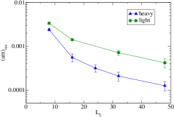
Figure 1: Residual quark mass as a function of $L_{5}$ for the two samples (heavy and light) of $25$ configurations each.

Furthermore, we require the absolute change in the masses of the pion and the nucleon under changes of $L_{5}$ to be small; these are shown in Figure 2 for the pion and nucleon masses. Note, that the errors are not independent between different points of $L_{5}$, since an identical sample of gauge field configurations has been used. Therefore, we have performed a separate analysis by Jackknifing the differences in the masses compared to $L_{5}=16$. The results are shown in Figure 3.

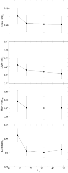
Figure 2: The pion mass with heavy and light quarks, $m_{\pi,\mbox{\tiny heavy}}$ and $m_{\pi,\mbox{\tiny light}}$, and the nucleon mass with heavy and light quarks, $m_{\mbox{\tiny N,heavy}}$ and $m_{\mbox{\tiny N,light}}$, as a function of $L_{5}$.

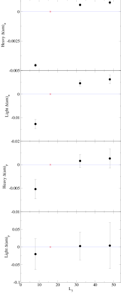
Figure 3: The same quantities as in Figure 2, but with a Jackknife analysis of the mass differences vs. $L_{5}=16$.

In the case of heavy quarks, the influence of increasing $L_{5}$ beyond $L_{5}=16$ is negligible in all observables. In the case of the light quarks, the influence is at most a few percent when going beyond $L_{5}=16$. Hence, we choose $L_{5}=16$ to be a good compromise between accuracy and performance.

2.2 Setting the quark mass

As outlined in the introduction, a necessary condition for a hybrid calculation to describe the physics of full QCD is that the masses of sea and valence quarks are identical.

Hence, we have chosen to match the pion masses of two different calculations: (i) full QCD calculations using three and two plus one flavors of dynamical Asqtad sea fermions and Asqtad valence fermions. These results have been taken from [9]. (ii) Our hybrid calculation with Asqtad dynamical sea fermions and valence domain-wall fermions with $L_{5}=16$.

To make the quark masses coincide, we tuned the bare mass parameter in the domain-wall valence fermion action so that the resulting pseudoscalar meson mass coincides with the corresponding meson mass in the Asqtad case. This condition is useful since the pseudoscalar meson mass is particularly sensitive to the choice of the quark mass.

The resulting choices for the bare quark masses, $(am)_{q}$, for Asqtad and domain-wall fermions are shown in Table 1. It is interesting that the difference between the bare quark masses for Asqtad and DWF valence quarks is quite substantial. Since this difference corresponds to the ratio of quark mass renormalization constants, we observe that either one or both of these renormalization constants deviates substantially from one.

Finally, we list the resulting nucleon masses — which we need for the calculation of the hadronic structure — in Table 2. There is a perceptible difference at the heaviest quark mass. The other masses are statistically compatible. Furthermore, there is no visible finite-size effect at the lightest quark mass. Thus, we only observe the expected ${\cal O}(a^{2})$ effects in the difference between the two masses at the heaviest quark mass.

Table 2: Nucleon masses as measured with Asqtad and domain-wall fermions for the valence quarks.

$\Omega$	$(am)_{q}^{\mbox{\tiny Asqtad,sea}}$	$(am)_{N}^{\mbox{\tiny Asqtad}}$	$(am)_{N}^{\mbox{\tiny DWF}}$
$20^{3}\times 32$	$0.050$	$1.057(5)$	$1.029(9)$
	$0.030/0.050$	$0.930(3)$	$0.941(10)$
	$0.010/0.050$	$0.779(6)$	$0.756(21)$
$28^{3}\times 32$	$0.010/0.050$		$0.763(12)$

3 HADRONIC STRUCTURE WITH LIGHT QUARKS

Within the framework discussed in the previous sections, we compute different observables of the nucleon structure for different quark masses. The results are compared to previous results from full QCD calculations with heavy quark masses, see References [10] for their calculation.

3.1 Form factor and transverse size of the proton

First, we consider the electromagnetic form factor $F_{1}(-t)$ of the nucleon. Phenomenologically, it follows a dipole-shaped behavior. Its derivative at the origin specifies the root-mean squared radius, $r_{\mbox{\tiny MS}}$, of the transverse charge distribution in the infinite-momentum frame and thus characterizes the size of of the nucleon. In a hypothetical world with heavy pions, the size of the nucleon should be smaller due to the absence of a significant pion cloud.

This qualitative behavior is well reproduced by our lattice data. Figure 4 shows our first results for the proton form factor, $F_{1}(-t)$. The triangles denote the heaviest quark mass in Table 1, the circles the intermediate quark mass of $(am)_{q}^{\mbox{\tiny Asqtad,sea}}=0.030/0.050$ and the boxes the lightest quark mass, all at the volume of $\Omega=20^{3}\times 32$. The dotted, the dashed, and the dash-dotted curves show the best dipole fit to these data points. The solid line shows the best dipole fit to the experimental data.

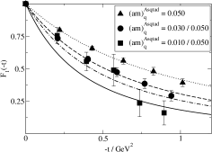
Figure 4: The proton form factor, $F_{1}(-t)$, as a function of the virtuality, $t=q^{2}$.

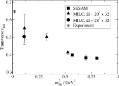
Figure 5: Transverse root-mean squared radius $r_{\mbox{\tiny MS}}$ of the nucleon as a function of the pion mass squared.

Figure 5 shows the transverse mean square radius, $r_{\mbox{\tiny MS}}$. The boxed data points represent the old SESAM data [10], obtained in a full QCD calculation with Wilson quarks. The triangular data points show the hybrid calculation with the data points from Table 1 with the volume $\Omega=20^{3}\times 32$. Finally, the circle represents the volume $\Omega=28^{3}\times 32$ in Table 1. As the quark mass decreases, the transverse size of the nucleon increases and approaches the experimental value. Note that we find no evidence of substantial finite-size corrections since there is no statistically significant difference between the data points at different volumes.

3.2 Axial charge

The axial charge, $g_{A}$, is given by the forward value of the generalized parton distribution $\tilde{A}_{1}^{\mbox{\tiny u-d}}$ (see Reference [6] for details). This quantity has been shown to exhibit substantial finite-size dependence [11] and therefore provides a good benchmark of the importance of the physical box size as we approach the chiral limit.

Figure 6 shows a central result of this work, the nucleon axial charge as a function of the pion mass squared. It has been renormalized using the five-dimensional conserved current. The symbols are the same as in Figure 5.

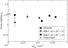
Figure 6: Nucleon axial charge, $g_{A}$, as a function of the pion mass squared.

We observe that the SESAM results in a $(1.6\,\mbox{fm})^{3}$ box first increase with decreasing pion mass and then fall off when the pion cloud becomes too large to fit in the box. In the larger $(2.6\,\mbox{fm})^{3}$ MILC box (on a $20^{3}$ lattice), the value at $m_{\pi}\simeq 700$ MeV increases back to its physical value again and then falls off at $m_{\pi}\simeq 300$ MeV when the light pion no longer fits in the box. Increasing the box to $(3.5\,\mbox{fm})^{3}$ ($28^{3}$ lattice) allows $g_{A}$ to increase to a physical value consistent with experiment. Thus, the locus of points in the largest box at each mass extrapolate smoothly to the experimental result.

To summarize, we give the resulting values of $r_{\mbox{\tiny MS}}$ and $g_{A}$ in Table 3.

Table 3: Summary of the hadron structure results. The table shows the volume, the Asqtad sea quark mass from Table 1, and the resulting values of $r_{\mbox{\tiny MS}}$ and $g_{A}$.

$\Omega$	$(am)_{q}^{\mbox{\tiny Asqtad,sea}}$	$r_{\mbox{\tiny MS}}$	$g_{A}$
$20^{3}\times 32$	$0.050$	$0.4113(14)$	$1.17(2)$
	$0.030/0.050$	$0.501(22)$	$1.20(4)$
	$0.010/0.050$	$0.551(80)$	$1.06(11)$
$28^{3}\times 32$	$0.010/0.050$	$0.503(46)$	$1.24(9)$

4 SUMMARY AND OUTLOOK

In this talk we have used a tuned hybrid calculation of Asqtad sea quarks and domain-wall valence quarks. We have determined an optimal value for $L_{5}$ in the domain-wall action and tuned the bare quark masses such that the pion masses of an Asqtad-valence and the domain-wall valence calculation agree. If the continuum limit exists, this calculation provides a valid scheme to compute all hadronic observables.

We have computed the $F_{1}(-t)$ form factor of the proton and obtained the $r_{\mbox{\tiny MS}}$ radius from it. The results are in qualitative agreement with the picture of the nucleon becoming larger as the pion cloud becomes more prominent with decreasing quark mass.

We have also applied our scheme to the case of the nucleon axial coupling, $g_{A}$. Whereas calculations in a fixed volume underestimate $g_{A}$ when the pion becomes too light to fit in the box, our sequence of calculations in three volumes produce a locus of points that smoothly extrapolate to the experimental result.

Encouraged by the successes reported here, we are continuing the calculation of hadronic observables using improved staggered sea quarks and domain-wall valence quarks.

References

- [1] W. Schroers et al., Nucl. Phys. Proc. Suppl. 106, 1082 (2002), F. Farchioni, C. Gebert, I. Montvay and W. Schroers, Nucl. Phys. Proc. Suppl. 106, 215 (2002), W. Schroers, Ph.D. thesis (2001) [arXiv:hep-lat/0304016].
- [2] C. T. H. Davies et al. [HPQCD Collaboration], Phys. Rev. Lett. 92, 022001 (2004).
- [3] K. Orginos, D. Toussaint and R. L. Sugar [MILC Collaboration], Phys. Rev. D 60, 054503 (1999), K. Orginos and D. Toussaint [MILC collaboration], Phys. Rev. D 59, 014501 (1999).
- [4] D. B. Kaplan, Phys. Lett. B 288, 342 (1992), V. Furman and Y. Shamir, Nucl. Phys. B 439, 54 (1995).
- [5] D. Müller, D. Robaschik, B. Geyer, F. M. Dittes and J. Horejsi, Fortsch. Phys. 42 (1994) 101, X. D. Ji, Phys. Rev. Lett. 78 (1997) 610, A. V. Radyushkin, Phys. Rev. D 56 (1997) 5524, M. Diehl, Phys. Rept. 388 (2003) 41.
- [6] M. Göckeler, R. Horsley, D. Pleiter, P.E.L. Rakow, A. Schäfer, G. Schierholz and W. Schroers [QCDSF collaboration], Phys. Rev. Lett. 92, 042002 (2004), P. Hägler, J.W. Negele, D.B. Renner, W. Schroers, T. Lippert and K. Schilling [LHP collaboration], Phys. Rev. D 68, 034505 (2003), W. Schroers et al. [LHP collaboration], Nucl. Phys. Proc. Suppl. 129, 907 (2004), P. Hägler, J.W. Negele, D.B. Renner, W. Schroers, T. Lippert and K. Schilling [LHP collaboration], Phys. Rev. Lett. (in print).
- [7] A. Hasenfratz and F. Knechtli, Phys. Rev. D 64 (2001) 034504.
- [8] T. Blum et al., Phys. Rev. D 69 (2004) 074502.
- [9] C. W. Bernard et al., Phys. Rev. D 64, 054506 (2001).
- [10] D. Dolgov et al. [LHP collaboration], Phys. Rev. D 66 (2002) 034506, J. W. Negele et al. [LHPC Collaboration], Nucl. Phys. Proc. Suppl. 129, 910 (2004), J. W. Negele et al., Nucl. Phys. Proc. Suppl. 128, 170 (2004).
- [11] S. Sasaki, K. Orginos, S. Ohta and T. Blum [the RIKEN-BNL-Columbia-KEK Collaboration], Phys. Rev. D 68, 054509 (2003).