Finite volume effects in chiral perturbation theory

Abstract

There has recently been an intense activity in the study of finite volume effects by means of chiral perturbation theory. In this contribution I review recent work in this field both for the $\epsilon$– ($M_{\pi}L\lesssim 1$) and the $p$–regime ($M_{\pi}L\gg 1$). For the latter I emphasize the importance of going beyond leading order calculations in chiral perturbation theory and the usefulness of asymptotic formulae à la Lüscher used in combination with CHPT.

1 Introduction

Every lattice calculation is done in finite volume and at finite lattice spacing, as well as at finite (and at present typically substantial) quark masses. Before being able to make a meaningful comparison to experimentally measured quantities, one has to make three extrapolations – and since all of them are numerically quite expensive, any analytical method that may help in this respect is more than welcome. Chiral perturbation theory (CHPT) provides the proper framework for calculating analytically the dependence on all three extrapolation parameters. An overview of the present status of the analytical calculations related to the extrapolation to the continuum and to the chiral limit, and in particular of the interplay between the two limits, has been given by Oliver Bär [1]. Here I will discuss the extrapolation to the infinite volume limit, and give an overview of the present status of analytical calculations in the framework of CHPT.

If a physical system is enclosed in a finite box, and periodic boundary conditions are imposed, the space of the possible three-momenta becomes discrete:

$$\vec{p}=\frac{2\pi}{L}\vec{n},\qquad\vec{n}=(n_{1},n_{2},n_{3})$$ (1)

with $n_{1,2,3}\in\mathbf{Z}$. If the box is large enough, this discrete space will almost look like a continuum one: and since one is interested in simulating the soft, nonperturbative dynamics of QCD, one would like to have the region of soft momenta to look like a continuum one. If we take $4\pi F_{\pi}$ as the chiral symmetry breaking scale, which separates soft from hard momenta, we obtain the following quantitative condition on the volume

$$\frac{2\pi}{L}\ll 4\pi F_{\pi}\qquad\Rightarrow\qquad L\gg\frac{1}{2F_{\pi}}\sim 1\,\mathrm{fm}$$ (2)

in order to have a large number and not only a few discrete momenta in the soft region.

If the condition (2) is satisfied one can then use CHPT to study analytically the behaviour of the system at low momenta, and in particular the explicit dependence of physical observables on the volume. How to extend the CHPT framework to the finite volume case has been discussed by Gasser and Leutwyler [2]: in finite volume CHPT becomes a systematic expansion in both the quark masses and the inverse box size. In infinite volume there are relations among the coefficients of this expansion for different quantities which follow from the chiral symmetry of QCD: these relations go traditionally under the name of “low energy theorems” and CHPT is a convenient tool to derive them systematically. In finite volume chiral symmetry implies relations among the coefficients of the expansion in $1/L$ of different observables as well as relations among these coefficients and those of the expansion in quark masses. CHPT allows one to obtain these “large volume theorems” in a systematic way.

The product $F_{\pi}L$ is not the only relevant parameter. An important role is also played by the relative size of $M_{\pi}$ and $1/L$. If $M_{\pi}L\lesssim 1$ finite volume effects will be similar to those in the chiral limit – as is well known, no spontaneous symmetry breaking can take place in a finite volume, and one will see a deformation of the vacuum state due to finite volume effects. If $M_{\pi}L\gg 1$, on the other hand, the effect of the explicit symmetry breaking on the low energy behaviour of the system will be more important than that due to the finite volume. In the framework of CHPT, the difference between the two situations is given by the importance that the Goldstone-boson zero modes have in the evaluation of the path integral. In the latter case, like in infinite volume, the contribution of the zero modes can be neglected, whereas in the first case is important and must be explicitly evaluated [2, 3]. The first situation is denoted as “$\epsilon$–regime” and the second one “$p$–regime”, and the respective counting schemes are as follows:

$$\epsilon\mbox{--regime:} M_{\pi}\sim\frac{1}{L^{2}}\sim O(\epsilon^{2})$$

$$p\mbox{--regime:} M_{\pi}\sim\frac{1}{L}\sim O(p)\;\;.$$ (3)

In the first case the Compton wavelength of the pion is larger than the box size, and the pion does not have enough space to propagate (all other non-Goldstone-like particles however do, because their mass is of the order of $\Lambda\sim 4\pi F_{\pi}$, and we assume that the condition (2) is satisfied). In the latter case, a pion fits comfortably well inside a box and, being the lightest particle, is the only one that has a nonnegligible probability to propagate until the box boundaries, and therefore feel their presence.

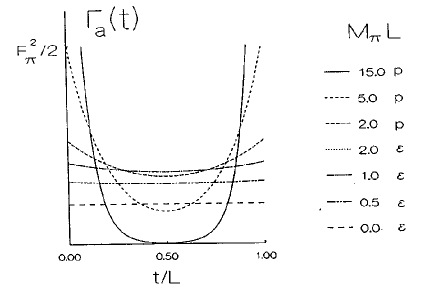
Figure 1: Time-dependence of the axial-charge correlator on for different values of $M_{\pi}L$. Note that for $M_{\pi}L=2$ the calculation in the $\epsilon$– and $p$–regime give perfectly overlapping results. Figure taken from [3]

The different behaviour of the physical system in the two cases is well illustrated in Fig. 1 where the time dependence of the correlator of two axial charges

$$\langle Q_{i}^{A}(t)Q_{k}^{A}(0)\rangle\equiv\delta_{ik}L^{3}\Gamma_{A}(t)$$ (4)

is plotted for different values of $M_{\pi}L$. In infinite volume the correlator drops exponentially with a rate which is proportional to $M_{\pi}$:

$$\Gamma_{A}^{L=\infty}(t)=M_{\pi}F_{\pi}^{2}/2\;e^{-M_{\pi}t}\left[1+O(p^{4})\right]\;\;.$$ (5)

In the $p$–regime one expects a behaviour of the correlator which is qualitatively similar to the one in infinite volume – as Fig. 1 indeed shows. In the $\epsilon$–regime, on the other hand, the qualitative behaviour is completely different from the infinite-volume case – the curves in Fig. 1 corresponding to small values of $M_{\pi}L$ can be well described by a polynomial of low degree in $t$ [3].

2 Finite volume effects in the $\epsilon$–regime

One of the goals of lattice calculations is to determine the low-energy constants of the CHPT Lagrangian. These constants are by definition independent of the light quark masses and a reliable determination should therefore be made with quark masses as small as possible, which is notoriously expensive. Even when very small masses will become accessible working close to the chiral limit and in the $p$–regime will require enormous volumes and will likely remain for a long time prohibitively expensive. Approaching the chiral limit on the lattice implies working in the $\epsilon$–regime. As discussed above, observable quantities may look very different in the $\epsilon$–regime from the infinite-volume case. The strategy of the calculation in this case must start from an analytical calculation in CHPT to identify the proper observable that will allow an extraction of the low-energy constant of interest. The first analytical calculations in this direction have been made in [3, 5]. The first numerical calculations which exploited this strategy were aimed at the extraction of the quark condensate in the chiral limit [6, 4].

More recently, two different groups engaged in the calculation of charge-charge correlators of the type defined in Eq. (4) in order to extract the pion decay constant in the chiral limit. Results have been published during last year [7, 8] and show a very clean determination of this chiral-limit observable. In fact one of the two groups has performed the calculation of the decay constant also in the $p$–regime and has shown that after the extrapolation to the chiral limit the result is in agreement with the direct determination in the $\epsilon$–regime:

$$F \simeq 130\;\,\mathrm{MeV}\hskip 127.18385pt\mbox{\cite[cite]{[\@@bibref{}{QQ1}{}{}]}}$$

$$F = (102\pm 4\;\,\mathrm{MeV})_{\epsilon}\;\;,\;\;\;(104\pm 2\;\,\mathrm{MeV})_{p}\quad\mbox{\cite[cite]{[\@@bibref{}{QQ2}{}{}]}}$$

Although the calculations have been made in the quenched approximation, the positive results prove the feasibility of the method and have opened the way for a more ambitious aim of the program: the calculation of the low-energy constant of the weak chiral Lagrangian for nonleptonic $K$-decays. The first results in this direction have been presented at this conference [9] and have also recently appeared [10].

Unfortunately, these groups have also found out that working in the $\epsilon$–regime is technically challenging, and to complete their program had to overcome unexpected, highly nontrivial difficulties of numerical nature [7, 8, 9]. It will be interesting to see the application of this strategy with dynamical fermions – which is certainly a highly nontrivial task.

Two papers have recently investigated this regime for the one-nucleon sector and promise interesting developments [11].

3 Finite volume effects in the $p$–regime

Gasser and Leutwyler [2] have shown that, if one works in the $p$–regime, in a large isotropic box with periodic boundary conditions, the only change in the calculation is that the propagator of the pseudo Goldstone bosons has to be made periodic:

$$G_{L}(\vec{x},t)=\sum_{\vec{n}}G_{\infty}(\vec{x}+\vec{n}L,t)\;\;.$$ (6)

The local vertices, as given by the CHPT Lagrangian, remain unchanged and the power counting for loop diagrams works like in infinite volume: every loop generates an additional $O(p^{2})$ correction. The only difference is that in finite volume $p\sim M\sim 1/L$, and a one-loop calculation gives both the leading quark-mass and finite volume corrections. For example, the one-loop calculation of $M_{\pi}$ and $F_{\pi}$ gives [2]:

$$M_{\pi}(L) = M_{\pi}\left[1+\frac{1}{2N_{f}}\xi\,g_{1}(\lambda)+O(\xi^{2})\right]$$

$$F_{\pi}(L) = \;F_{\pi}\left[1-\;\frac{N_{f}}{2}\,\xi\,g_{1}(\lambda)+O(\xi^{2})\right]$$ (7)

with $\lambda=M_{\pi}L$, $\xi=(M_{\pi}/4\pi F_{\pi})^{2}$ and

$$g_{1}(\lambda) = \sum_{\vec{n}}\nolimits^{\prime}\int_{0}^{\infty}dz\;e^{-{1\over z}-\frac{z}{4}\vec{n}^{2}\lambda^{2}}$$ (8)

$$= \sum_{k=1}^{\infty}\frac{4m(k)}{\sqrt{k}\lambda}K_{1}(\sqrt{k}\lambda)\;\;,$$

is the tadpole correction in finite volume ($m(k)$ is the multiplicity of a vector $\vec{n}$ with $\vec{n}^{2}=k$). The result shows that finite volume corrections for masses and decay constants are suppressed exponentially, by increasing powers of $\exp(-M_{\pi}L)$. The infinite sum appearing in Eq. (8) reflects the infinite sum in the definition of a fully periodic propagator, Eq. (6), but since $M_{\pi}L\gg 1$ only the first few will be numerically relevant.

A different approach which relies on an expansion in exponentials and not on CHPT is due to Lüscher [12] – this expansion, however, has only been devised for masses and, more recently, for decay constants [13], and is therefore less general than the chiral expansion. A detailed comparison of the two approaches will be given later.

3.1 Overview of recent results

The examples just discussed show that, in the $p$–regime finite-volume effects are typically small and relevant for very precise lattice calculations. Indeed only recently there has been an intense activity in analytical calculations of these effects despite the fact that the theoretical framework had been established around twenty years ago [2, 12], and extended to the quenched approximation not much later [14, 15].

During last year there have been analyses of finite volume effects for: two-pion state energies [16], the pion mass [17], $F_{K}$ and $B_{K}$ [18], the nucleon mass [19, 20], the nucleon magnetic moments and axial coupling constant as well as the mass [21], $f_{B}$ and $B_{B}$ [22] and $F_{\pi}$ [13]. Many of these results have been also presented at this conference [23, 24, 25] together with new ones concerning $M_{\pi},\;F_{\pi}$ and the charge radius [26]. Most of these calculations have been made in the framework of CHPT and concerned one-loop finite-volume effects and not using Lüscher formula. A comparison to the Lüscher formula has been made in the case of the proton mass [19], and a discrepancy has been found with the explicit formula given by Lüscher in his Cargèse lecture notes [27]. It turns out that the formula in these lecture notes was not correctly written and that the correction has numerically important effects (cf. [19, 20]).

In what follows I will discuss in some more detail why it is important to go beyond the leading-order calculation of these effects if one wants to have a good control over them, and how this can be achieved by a combined use of CHPT and the asymptotic formulae à la Lüscher. This is the approach advocated in [17, 13].

3.2 Hadron masses in finite volume: CHPT vs. Lüscher Formula

Above we have briefly discussed what rules one has to follow if one wants to calculate finite volume corrections to a given quantity in CHPT, and shown the result for the pion mass. The analogous result for the kaon, the proton or any other hadron mass will of course be different. Lüscher, however, has shown that the leading exponential correction to the mass of a given hadron can be expressed in a completely universal way through an integral over the scattering amplitude of the hadron in question and the pion. The latter enters here because it is the lightest hadron: the leading exponential correction to any hadron mass is of the form $\exp(-M_{\pi}L)$, and how large the correction is depends on how strong is the interaction of the hadron in question to the pion. For example the Lüscher formula for the pion mass reads

$$M_{\pi}(L)-M_{\pi}=-\frac{3}{16\pi^{2}M_{\pi}L}\times\hskip 56.9055pt$$ (9)

$$\int_{-\infty}^{\infty}\!dy\;F({\rm i}y)\,e^{-\sqrt{M_{\pi}^{2}+y^{2}}\,L}+O(e^{-\overline{M}L})$$

where $F(\nu)$ is the physical (for $\nu$ real – what enters the integral is the analytic continuation) forward $\pi\pi$ scattering amplitude and $\overline{M}>\sqrt{2}M_{\pi}$. Note that the formula does not rely in any way on the chiral expansion, and indeed is valid also in cases where there is no spontaneous symmetry breaking and the corresponding Goldstone bosons – in such cases the role of the pion has to be overtaken by the particle which happens to be the lightest one.

The formula can be used for a numerical analysis only if one has a representation for the scattering amplitude in the integrand which lends itself to a numerical evaluation. For hadrons one could in principle take directly the measured scattering amplitude (and do the necessary analytic continuation) to evaluate the integral, but then one would be restricted to physical values of the quark masses: in order to use the formula for arbitrary values of the quark masses one must therefore rely on the chiral representation for the scattering amplitude. Inserting the leading order chiral representation for the $\pi\pi$ scattering amplitude:

$$F(\nu)=-\frac{M_{\pi}^{2}}{F_{\pi}^{2}}+O(M_{\pi}^{4})$$ (10)

in Eq. (9) one should obtain the same expression for the leading exponential term in Eq. (7). As was verified long ago [2], this is indeed the case.

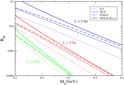
Figure 2: Relative finite volume corrections ($R_{M}=(M_{\pi,L}-M_{\pi})/M_{\pi}$) to the pion mass using the Lüscher formula (9) or the modified version which includes subleading exponentials (11) and the chiral expansion of the $\pi\pi$ amplitude up to NNLO.

The chiral expansion for the scattering amplitude is now known up to and including order $p^{6}$ [28], and it is easy to insert the corresponding analytic expressions in Eq. (9) and evaluate the integral. This has been done in [17], and the corresponding numerical results are shown in Fig. 2. A somewhat surprising feature of the numerical results is that the NLO corrections are quite substantial and of the order of 50% of the LO effect. The comparison of NLO and NNLO however shows that chiral expansion does have a good converging behaviour for all values of $M_{\pi}$ and $L$ in the region of applicability of the formula.

A comparison to the numerical values obtained with the full one-loop CHPT formula Eq. (7) on the other hand shows that for not so large values of $M_{\pi}L$ exponentially subleading terms may be important. As was suggested in [17] the most reliable estimate of the finite volume effects for the pion mass is obtained by adding to the full one-loop CHPT result the NLO and NNLO corrections obtained through the Lüscher formula. There is actually a simple extension of the Lüscher formula that provides a convenient combination of both approaches. The modified formula is the following:

$$M_{\pi,L}-M_{\pi}=-\frac{1}{32\pi^{2}\lambda}\sum_{k=1}^{\infty}{m(k)\over\sqrt{k}}\times$$ (11)

$$\int_{-\infty}^{\infty}dyF(iy)e^{-\sqrt{k(M_{\pi}^{2}+y^{2})}L}+O(e^{-\overline{M}L})$$

and can be derived with the following reasoning. In Lüscher’s paper [12] a substantial part of the proof of the formula is devoted to showing that the leading exponential corrections are obtained from loop graphs where only one pion propagator is taken in finite volume (i.e. is made periodic, as in Eq. (6)) and all other propagators are the standard, infinite-volume ones. Since he concentrates only on the leading exponential correction, he then immediately drops all terms with $|\vec{n}|>1$ in the infinite sum which makes the propagator periodic. But nothing forbids to keep all terms in the infinite sum Eq. (6) and to follow the rest of the derivation which leads to Eq. (11).

A few comments are in order:

1. although Eq. (11) contains exponentially subleading terms, it is not algebraically better than Eq. (9) because both give only the leading term exactly – numerically, however, the effect of subleading terms is important for moderate values of $M_{\pi}L$ as shown in Fig. 2;

2. an inclusion of exponentially subleading terms which is similar in spirit to the one proposed here has been already introduced by Lüscher by extending the integration boundaries to infinity in Eq. (9);

3. at the two-loop level there will be two types of contributions which are not included in Eq. (11): contributions where two pion propagators are taken in finite volume, and contributions to the loop integration from other singularities other than the pion pole in the propagator (note that both contributions are absent at the one-loop level: indeed if one inserts the leading order amplitude (10) in Eq. (11) one recovers exactly the full one-loop result (7)). Only a complete two-loop calculation will show how big these contributions are numerically [29].

3.3 Decay constants in finite volume

The discussion in the previous subsection has shown the usefulness of the asymptotic formula of Lüscher in evaluating finite-volume corrections for masses, and calls for extensions to other quantities. Recently, an extension to decay constants has been provided in [13] and reads

$$F_{\pi,L}-F_{\pi}=\frac{3}{8\pi^{2}M_{\pi}L}\times$$

$$\int_{-\infty}^{\infty}dy\;e^{-\sqrt{M_{\pi}^{2}+y^{2}}L}N_{F}(iy)+O(e^{-\bar{M}L})\;\;,$$ (12)

where $N_{F}(\nu)$ is (as one intuitively expects) related to the $\langle 0|A_{\mu}|3\pi\rangle$ amplitude. In this case there is a subtlety related to the fact that the latter amplitude has a pole due to the direct coupling of the axial current to a pion, which then rescatters into three pions. This pole appears exactly in the kinematical region where it is needed in Eq. (12) and must be subtracted. The prescription for the subtraction of this pole has been discussed in detail in [13], together with the physical interpretation of the subtraction.

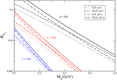
Figure 3: Relative finite volume corrections to the pion decay constant ($R_{F_{\pi}}=(F_{\pi,L}-F_{\pi})/F_{\pi}$).

This asymptotic formula can now be used for a numerical analysis in the same way as the Lüscher formula for the pion mass: in the present case the needed infinite-volume amplitude is the one relevant for the decay of the $\tau$ into a neutrino and three pions and has been calculated to one loop in CHPT [30]. The numerical results, including the effects of subleading exponential terms, included according to the analogous of Eq. (11) are shown in Fig. 3.

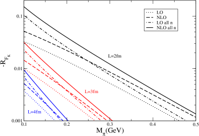
Figure 4: Relative finite volume corrections to the kaon decay constant ($R_{F_{K}}=(F_{K,L}-F_{K})/F_{K}$).

Like Lüscher’s formula, this extension to decay constants can also be applied to heavier hadrons: what determines the finite-volume correction to the decay constant of the hadron H is the amplitude $\langle 0|A_{\mu}|2\pi H\rangle$. For the case of the kaon, e.g., this is the amplitude relevant for $K_{l4}$ decays, which is nowadays known to two loops [31]. A numerical analysis based on the one-loop evaluation of this amplitude [32] gives the results shown in Fig. 4. Finite volume corrections for $F_{\pi}$ and $F_{K}$ are also of phenomenological interest, because the lattice calculation of these two quantities can be used to determine $V_{us}$, as suggested by Marciano [33], and performed by the MILC collaboration [34]. A complete numerical analysis of the masses and decay constants of all the octet of pseudoscalars is in progress [29].

4 Conclusions

There has been a lot of activity recently in calculating finite volume effects analytically. I have briefly reviewed the theoretical tools needed for performing these calculations as well as some of this recent activity. The cost of a lattice calculation grows very rapidly with the box size – the calculations discussed here show that in many cases it is unnecessary to make the infinite-volume extrapolation numerically, and one can correct for finite-volume effects analytically.

References

- [1] Oliver Bär, these Proceedings.
-
[2]
J. Gasser and H. Leutwyler,
Nucl. Phys. B 307 (1988) 763,
Phys. Lett. B 184 83 (1987),
Phys. Lett. B 188 (1987) 477;
H. Leutwyler, Phys. Lett. B 189 (1987) 197. -
[3]
F. C. Hansen,
Nucl. Phys. B 345 (1990) 685;
F. C. Hansen and H. Leutwyler, Nucl. Phys. B 350 (1991) 201. - [4] P. Hasenfratz et al. Nucl. Phys. B 643 (2002) 280 [arXiv:hep-lat/0205010].
- [5] H. Leutwyler and A. Smilga, Phys. Rev. D 46 (1992) 5607.
- [6] P. Hernandez, K. Jansen and L. Lellouch, Phys. Lett. B 469 (1999) 198 [arXiv:hep-lat/9907022].
- [7] W. Bietenholz, T. Chiarappa, K. Jansen, K. I. Nagai and S. Shcheredin, JHEP 0402 (2004) 023 [arXiv:hep-lat/0311012].
- [8] L. Giusti et al. JHEP 0404 (2004) 013 [arXiv:hep-lat/0402002].
- [9] Hartmut Wittig, these Proceedings.
-
[10]
L. Giusti et al.
arXiv:hep-lat/0407007,
L. Giusti et al. arXiv:hep-lat/0409031. -
[11]
W. Detmold and M. J. Savage,
arXiv:hep-lat/0407008;
P. F. Bedaque, H. W. Griesshammer and G. Rupak, arXiv:hep-lat/0407009. - [12] M. Lüscher, Commun. Math. Phys. 104, 177 (1986).
- [13] G. Colangelo and C. Haefeli, Phys. Lett. B 590 (2004) 258 [arXiv:hep-lat/0403025].
- [14] C. W. Bernard and M. F. L. Golterman, Phys. Rev. D 46 (1992) 853 [arXiv:hep-lat/9204007]; Phys. Rev. D 53 (1996) 476 [arXiv:hep-lat/9507004].
- [15] S. R. Sharpe, Phys. Rev. D 46 (1992) 3146 [arXiv:hep-lat/9205020].
- [16] C. J. D. Lin et al. Phys. Lett. B 581 (2004) 207 [arXiv:hep-lat/0308014].
- [17] G. Colangelo and S. Durr, Eur. Phys. J. C 33 (2004) 543 [arXiv:hep-lat/0311023].
- [18] D. Becirevic and G. Villadoro, Phys. Rev. D 69 (2004) 054010 [arXiv:hep-lat/0311028];
- [19] A. Ali Khan et al. [QCDSF-UKQCD Coll.], arXiv:hep-lat/0312030.
- [20] Y. Koma and M. Koma, arXiv:hep-lat/0406034.
-
[21]
S. R. Beane,
Phys. Rev. D 70 (2004) 034507
[arXiv:hep-lat/0403015];
S. R. Beane and M. J. Savage, arXiv:hep-ph/0404131. - [22] D. Arndt and C. J. D. Lin, arXiv:hep-lat/0403012.
- [23] D. Lin, these proceedings.
- [24] M. Goeckeler, these proceedings.
- [25] Y. Koma and M. Koma, these proceedings [arXiv:hep-lat/0409002].
- [26] B. Borasoy, R. Lewis and D. Mazur, these proceedings [arXiv:hep-lat/0408040].
- [27] M. Luscher, DESY 83/116 Lecture given at Cargese Summer Inst., Cargese, France, Sep 1-15, 1983
- [28] J. Bijnens et al., Phys. Lett. B 374 210 (1996) [arXiv:hep-ph/9511397], Nucl. Phys. B 508 263 (1997) [Erratum-ibid. B 517 639 (1998)] [arXiv:hep-ph/9707291].
- [29] G. Colangelo and C. Haefeli, in progress.
- [30] G. Colangelo, M. Finkemeier and R. Urech, Phys. Rev. D 54 (1996) 4403 [arXiv:hep-ph/9604279].
- [31] G. Amoros, J. Bijnens and P. Talavera, Nucl. Phys. B 585 (2000) 293 [Erratum-ibid. B 598 (2001) 665] [arXiv:hep-ph/0003258].
- [32] J. Bijnens, G. Colangelo and J. Gasser, Nucl. Phys. B 427 (1994) 427 [arXiv:hep-ph/9403390].
- [33] W. J. Marciano, arXiv:hep-ph/0402299.
- [34] C. Aubin et al. [MILC Collaboration], arXiv:hep-lat/0407028.