Detailed analysis of the gluonic excitation in the three-quark system in lattice QCD

Abstract

We study the excited-state potential and the gluonic excitation in the static three-quark (3Q) system using SU(3) lattice QCD with $16^{3}\times 32$ at $\beta$=5.8 and 6.0 at the quenched level. For about 100 different patterns of spatially-fixed 3Q systems, we accurately extract the excited-state potential $V_{\rm 3Q}^{\rm e.s.}$ together with the ground-state potential $V_{\rm 3Q}^{\rm g.s.}$ by diagonalizing the QCD Hamiltonian in the presence of three quarks. The gluonic excitation energy $\Delta E_{\rm 3Q}\equiv V_{\rm 3Q}^{\rm e.s.}-V_{\rm 3Q}^{\rm g.s.}$ is found to be about 1 GeV at the typical hadronic scale. This large gluonic-excitation energy is conjectured to give a physical reason of the success of the quark model for low-lying hadrons even without explicit gluonic modes. We investigate the functional form of $\Delta E_{\rm 3Q}$ in terms of the 3Q location. The lattice data of $\Delta E_{\rm 3Q}$ are relatively well reproduced by the “inverse Mercedes Ansatz” with the “modified Y-type flux-tube length”, which indicates that the gluonic-excitation mode is realized as a complicated bulk excitation of the whole 3Q system.

I Introduction

It is widely accepted that quantum chromodynamics (QCD) QCD6673 is the fundamental theory of the strong interaction for hadrons and nuclei. Nevertheless, it still remains as a difficult problem to derive low-energy physical quantities directly from QCD in an analytic manner. The perturbative QCD calculation, which successfully describes the high-energy process, cannot be applied at the hadronic scale, since the QCD coupling constant becomes large in the infrared region. Furthermore, the strong-coupling nature of QCD leads to a highly nontrival vacuum with rich nonperturbative phenomena such as color confinement and spontaneous chiral symmetry breaking.

In this decade, the lattice-QCD Monte Carlo calculation has been recognized as a reliable nonperturbative method for the quantitative analysis of QCD, and the nonperturbative analysis based on QCD has become one of the central and important issues in the hadron physics. For instance, lattice QCD calculations successfully reproduce hadron mass spectra CPPACS01 and also predict the QCD phase transition at finite temperatures and densities K03 . On the other hand, the underlying structure of hadrons is not yet well investigated using lattice QCD. In fact, the application of lattice QCD is just beginning for the research of the hadron structure and related excitation modes in terms of quarks and gluons.

The investigation on the hadron structure and the excitation modes has a long history in the particle physics. In 1969, Y. Nambu first pointed out the string picture for hadrons N69 ; N70 to explain the Veneziano amplitude V68 on hadron reactions and resonances. Since then, the string picture has been one of the most important scenarios for hadrons N74 ; KS75 and has provided many interesting ideas in the wide region of the elementary particle physics P98 . For instance, the hadronic string creates infinite number of hadron resonances as the vibrational modes, and these excitations lead to the Hagedorn “ultimate” temperature H65 ; P84 , which gives an interesting theoretical picture for the QCD phase transition.

For real hadrons, the hadronic string has a spatial extension like a “flux-tube” N74 ; CNN79 ; CI86 ; SST95 , as the result of one-dimensional squeezing of the color-electric flux in accordance with color confinement N74 ; SST95 . Therefore, the vibrational modes of the hadronic flux-tube should be much more complicated, and the analysis of the excitation modes is important to clarify the underlying picture for real hadrons.

In the language of QCD, such non-quark-origin excitation is called as the “gluonic excitation” TS03 ; SIT04 ; JKM03 , and is physically interpreted as the excitation of the gluon-field configuration in the presence of the quark-antiquark pair or the three quarks in a color-singlet state.

In the hadron physics, the gluonic excitation is one of the interesting phenomena beyond the quark model, and relates to the hybrid hadrons such as $q\bar{q}G$ and $qqqG$ in the valence picture. For instance, the hybrid meson includes the exotic hadrons with the exotic quantum number such as $J^{PC}=0^{--},0^{+-},1^{-+},2^{+-},\cdots$, which cannot be constructed in the simple quark model DGH92 . Then, it is important to investigate the gluonic excitation with lattice QCD, not only from the theoretical viewpoint but also from the experimental viewpoint.

In this paper, we study the excited-state three-quark (3Q) potential and the gluonic excitation in baryons using lattice QCD TS03 , to get deeper insight on these excitations beyond the hypothetical models such as the string and the flux-tube models. In QCD, the excited-state 3Q potential is defined as the energy of the excited state of the gluon-field configuration in the presence of the static three quarks, and the gluonic-excitation energy is expressed as the energy difference between the ground-state 3Q potential TMNS99 ; TMNS01 ; TSNM02 and the excited-state 3Q potential.

Note that the inter-quark potential is one of the most fundamental quantities directly connected to color confinement, and plays the important role for hadron properties. As for the Q-$\rm\bar{Q}$ system, a lot of lattice QCD studies C7980 ; BS92 ; B01 ; LW01 have shown that the ground-state Q-$\rm\bar{Q}$ potential $V_{\rm Q\bar{Q}}^{\rm g.s.}$ is well described by the Coulomb plus linear potential, $V_{\rm Q\bar{Q}}^{\rm g.s.}=-\frac{A_{\rm Q\bar{Q}}}{r}+\sigma_{\rm Q\bar{Q}}r+C_{\rm Q\bar{Q}},$ with the inter-quark distance $r$. Its behavior at short distances can be explained by the Coulomb interaction from the one-gluon-exchange (OGE) process, and the linear confinement term seems to indicate the flux-tube picture N74 ; CNN79 , where the quark and the antiquark are linked by one dimensional flux-tube with the string tension of $\sigma\simeq 0.89$ GeV/fm.

In QCD, the three-body force among three quarks is also a “primary” force reflecting the SU(3) gauge symmetry, while the three-body force is regarded as a residual interaction in most fields in physics. In fact, the 3Q potential is directly responsible for the structure and properties of baryons, similar to the relevant role of the Q-$\bar{\rm Q}$ potential for meson properties, and both the Q-$\bar{\rm Q}$ potential and the 3Q potential are equally important fundamental quantities in QCD. Furthermore, the 3Q potential is the key quantity to clarify the quark confinement mechanism in baryons. However, in contrast with the Q-$\rm\bar{Q}$ potential, there were only a few preliminary lattice-QCD works SW8486 ; KEFLM87 ; TES88 done in 1980’s for the ground-state 3Q potential before our first study in 1999 TMNS99 .

Since 1999, we have performed accurate calculations and detailed analyses of the ground-state 3Q potential $V_{\rm 3Q}^{\rm g.s.}$ in lattice QCD with the smearing method for more than 300 different patterns of 3Q systems TSNM02 . In Refs. TMNS99 ; TMNS01 ; TSNM02 , we have shown that the ground-state 3Q potential $V_{\rm 3Q}^{\rm g.s.}$ is well described by the Coulomb plus Y-type linear potential, i.e., the Y-Ansatz,

$$V_{\rm 3Q}^{\rm g.s.}=-A_{\rm 3Q}\sum_{i<j}\frac{1}{|{\bf r}_{i}-{\bf r}_{j}|}+\sigma_{\rm 3Q}L_{\rm min}+C_{\rm 3Q},$$ (1)

within 1%-level deviation. Here, $L_{\rm min}$ denotes the minimal value of the total length of color-flux-tubes linking the three quarks CI86 ; TMNS99 ; TMNS01 ; TSNM02 ; FRS91 ; BPV95 , which is schematically illustrated in Fig. 1. We have found two remarkable features, the universality of the string tension as $\sigma_{\rm 3Q}\simeq\sigma_{\rm Q\bar{Q}}$ and the OGE result as $A_{\rm 3Q}\simeq\frac{1}{2}A_{\rm Q\bar{Q}}$. (Very recently, we show that the multi-quark potential is well described by the OGE Coulomb plus multi-Y type linear potential OST04 , which also supports the Y-Ansatz.)

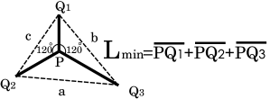
Figure 1: The Y-type flux-tube configuration of the 3Q system with the minimal value of the total flux-tube length, $L_{\rm min}=\sum_{i=1}^{3}\overline{\rm PQ}_{i}$. There appears a physical junction linking the three flux tubes at the Fermat point P.

We briefly summarize several other recent studies on the ground-state 3Q potential to clarify the current status of the Y-Ansatz.

After our first study, de Forcrand’s group tested only about 20 equilateral 3Q configurations in lattice QCD, and supported the $\Delta$-Ansatz AdFT02 . However, their data seem to indicate the Y-Ansatz with an overall constant shift, and the deviation seems to originate from the data at very short distances, where the linear potential is negligible compared with the Coulomb contribution. (Also, their usage of the continuum Coulomb potential may be problematic for the lattice data at very short distances.) Recently, de Forcrand’s group seems to change their opinion from the $\Delta$-Ansatz to the Y-Ansatz JdF03 .

One of the theoretical basis of the $\Delta$-Ansatz was Cornwall’s conjecture based on the vortex vacuum model C96 . Very recently, motivated by our studies, Cornwall re-examined his previous work and found an error in the model calculation. The corrected answer was the Y-Ansatz instead of the $\Delta$-Ansatz C04 .

As another analytical work, Kuzmenko and Simonov also showed that the Delta-shape is impossible from gauge-invariance point of view, and the Y-shaped configuration is the only possible for the 3Q system KS03 .

As a clear evidence for the Y-Ansatz, Ichie et al. performed the direct measurement on the action density in the spatially-fixed 3Q system in lattice QCD using the maximally-Abelian projection, and observed a clear Y-type flux-tube profile IBSS03 ; SIT04 .

In this way, the Y-Ansatz is also supported by various studies of other groups JdF03 ; KS03 ; C04 ; IBSS03 , and therefore the Y-Ansatz for the ground-state 3Q potential is almost settled both in lattice QCD and in analytic framework.

As for the excited-state 3Q potential, however, there is no lattice QCD study besides our previous work TS03 . In this paper, we present the detailed analysis of the excited-state 3Q potential and the gluonic excitation for about 100 different patterns of the 3Q static systems in SU(3) lattice QCD at the quenched level.

This paper is organized as follows. In section II, we give a necessary formalism on the relation between the 3Q Wilson loop and the QCD Hamiltonian. We then give the lattice QCD formalism to extract the excited-state 3Q potential in section III, and show the lattice QCD results in section IV. In section V, we investigate the functional form of the gluonic excitation energy from the lattice QCD data. In section VI, we discuss the physical implication of the obtained lattice results, and consider the physical reason of the success of the quark model for low-lying hadrons in terms of the gluonic excitation. Section VII is devoted to the summary and the conclusion.

II 3Q Wilson loop and 3Q potentials

II.1 3Q Wilson loop and QCD Hamiltonian

To begin with, let us consider the physical modes in the static 3Q system. We denote the $n$th excited state by $|n\rangle$ ($n$=0,1,2,3,..) for the physical eigenstates of the QCD Hamiltonian $\hat{H}$ for the spatially-fixed 3Q system. For the simple notation, the ground state is expressed as the “0th excited state” in this paper. Since the three quarks are spatially fixed in this case, the eigenvalue of $\hat{H}$ is expressed by the static 3Q potential as

$$\hat{H}|n\rangle=E_{n}|n\rangle=V_{n}|n\rangle,$$ (2)

where $V_{n}$ denotes the $n$th excited-state 3Q potential. We take the normalization condition as $\langle m|n\rangle=\delta_{mn}$. Note that both $V_{n}$ and $|n\rangle$ are universal physical quantities related to the QCD Hamiltonian $\hat{H}$.

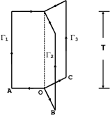
Figure 2: The 3Q Wilson loop $W_{\rm 3Q}$. The gauge-covariant 3Q state $|\Phi\rangle$ is generated at $t=0$ and is annihilated at $t=T$. The three quarks are spatially fixed in ${\bf R}^{3}$ for $0<t<T$.

Similar to the calculation of the Q-${\rm\bar{Q}}$ potential with the Wilson loop, the 3Q potential can be calculated with the 3Q Wilson loop $W_{\rm 3Q}$ defined as

$$W_{\rm 3Q}\equiv\frac{1}{3!}\varepsilon_{abc}\varepsilon_{a^{\prime}b^{\prime}c^{\prime}}U_{1}^{aa^{\prime}}U_{2}^{bb^{\prime}}U_{3}^{cc^{\prime}}$$ (3)

with $U_{k}\equiv P\exp\{ig\int_{\Gamma_{k}}dx^{\mu}A_{\mu}(x)\}$ ($k=1,2,3$). Here, $P$ denotes the path-ordered product along the path denoted by ${\Gamma_{k}}$ in Fig. 2.

In the 3Q Wilson loop, a gauge-covariant 3Q state $|\Phi\rangle$ is generated at $t=0$ and is annihilated at $t=T$ with the three quarks being spatially fixed in ${\bf R}^{3}$ for $0<t<T$. In general, the 3Q state $|\Phi\rangle$ in the 3Q Wilson loop is not an eigenstate of the QCD Hamiltonian $\hat{H}$ for the spatially-fixed 3Q system, and can be expressed with a linear combination of the 3Q physical eigenstates $|n\rangle$ ($n$=0,1,2..) as

$$|\Phi\rangle=c_{0}|0\rangle+c_{1}|1\rangle+c_{2}|2\rangle+..,$$ (4)

where the complex coefficients $c_{n}$ satisfy $\sum_{n=1}^{\infty}|c_{n}|^{2}=1$ and express the overlap with each state $|n\rangle$ in the 3Q Wilson loop.

Since the Euclidean time evolution of the 3Q state $|\Phi(t)\rangle$ is expressed with the operator $e^{-\hat{H}t}$, which corresponds to the transfer matrix in lattice QCD, the expectation value of the 3Q Wilson loop is expressed as

$$\langle W_{\rm 3Q}(T)\rangle=\langle\Phi(T)|\Phi(0)\rangle=\langle\Phi|e^{-\hat{H}T}|\Phi\rangle$$ (5)

$$=\sum_{m=0}^{\infty}\sum_{n=0}^{\infty}\bar{c}_{m}c_{n}\langle m|e^{-\hat{H}T}|n\rangle=\sum_{n=0}^{\infty}|c_{n}|^{2}e^{-V_{n}T}.$$

Then, the low-lying potentials, e.g., the ground-state potential $V_{\rm 3Q}^{\rm g.s.}\equiv V_{0}$ and the 1st excited-state potential $V_{\rm 3Q}^{\rm e.s.}\equiv V_{1}$, can be obtained from the large-$T$ behavior of $\langle W_{\rm 3Q}(T)\rangle$ where higher excited-state contributions are negligible. In practical lattice simulations, however, it is difficult to calculate $\langle W_{\rm 3Q}(T)\rangle$ accurately for large $T$, since its value decreases exponentially with $T$.

Therefore, for the accurate calculation of low-lying potentials, it is desired to reduce higher excited-state components in the 3Q state $|\Phi\rangle$ in the 3Q Wilson loop.

II.2 The smearing method

For this purpose, we use the smearing method APE87 to reduce highly excited-state components in the 3Q state $|\Phi\rangle$. The smearing is just a method for the state composition in a gauge-covariant manner, and never changes physical quantities and gauge configurations, unlike the cooling.

The smearing for link-variables is expressed as the iterative replacement of the spatial link-variable $U_{i}(s)$ ($i=1,2,3$) by the obscured link-variable $\bar{U}_{i}(s)\in{\rm SU(3)}$ which maximizes

$${\rm Re}\,\,{\rm tr}\Bigg{\{}\bar{U}_{i}^{\dagger}(s)\Bigg{[}\alpha U_{i}(s)+\sum_{j\neq i}\{U_{j}(s)U_{i}(s+\hat{j})U_{j}^{\dagger}(s+\hat{i})$$

$$\quad\quad\quad+U_{j}^{\dagger}(s-\hat{j})U_{i}(s-\hat{j})U_{j}(s+\hat{i}-\hat{j})\}\Bigg{]}\Bigg{\}},$$ (6)

leaving the temporal link-variable $U_{4}(s)$ unchanged.

Note that the smeared 3Q Wilson loop composed by the smeared link-variable is expressed as a spatially-extended operator in terms of the original link-variable $U_{\mu}(s)$, and therefore the 3Q state $|\Phi\rangle$ and the coefficients $c_{n}$ in the smeared 3Q Wilson loop are changed according to the iteration number $N_{\rm smr}$ of the smearing. In other words, the coefficients $c_{n}$ in the smeared 3Q Wilson loop can be controlled to some extent in the smearing procedure, by changing the iteration number $N_{\rm smr}$ and the smearing parameter $\alpha$.

For instance, as the iteration number $N_{\rm smr}$ of the smearing increases from $N_{\rm smr}$=0, the excited-state components in the $N_{\rm smr}{\rm th}$ smeared 3Q Wilson loop gradually decrease, and finally the 22th (42th) smeared 3Q Wilson loop is almost ground-state saturated as $|\Phi\rangle\simeq c_{0}^{k}|0\rangle$ for $\alpha=2.3$ on the lattice with $\beta$=5.8 (6.0) TSNM02 . Then, with the properly smeared 3Q Wilson loop $\langle W_{\rm 3Q}(T)\rangle$, $V_{\rm 3Q}^{\rm g.s.}$ can be accurately calculated as $V_{\rm 3Q}^{\rm g.s.}\simeq-\frac{1}{T}\ln\langle W_{\rm 3Q}(T)\rangle$ even at relatively small $T$ TMNS01 ; TSNM02 .

The smearing method is also useful to extract the low-lying 3Q potentials, i.e., the ground-state potential $V_{\rm 3Q}^{\rm g.s.}$ and the 1st excited-state potential $V_{\rm 3Q}^{\rm e.s.}$ TS03 ; SIT04 .

III Formalism

In this section, we present the formalism of the variational method TS03 ; LW90 ; PM90 to extract the excited-state potential and the gluonic excitation by diagonalizing the QCD Hamiltonian in the presence of static quarks.

Suppose that $|\Phi_{k}\rangle\ (k=0,1,2,3,..)$ are arbitrary given independent 3Q states for the spatially-fixed 3Q system. In general, each 3Q state $|\Phi_{k}\rangle$ can be expressed with a linear combination of the 3Q physical eigenstates $|n\rangle\ (n=0,1,2,..)$ as

$$|\Phi_{k}\rangle=c_{0}^{k}|0\rangle+c_{1}^{k}|1\rangle+c_{2}^{k}|2\rangle+..$$ (7)

Here, the coefficients $c_{n}^{k}$ depend on the selection of the 3Q states $|\Phi_{k}\rangle$, and hence they are not universal quantities. (Unlike the Q-$\bar{\rm Q}$ system, there is no definite symmetry in the 3Q system, so that we do not construct the 3Q states which carry the specific quantum number.)

The Euclidean time-evolution of the 3Q state $|\Phi(t)\rangle$ is expressed with the operator $e^{-\hat{H}t}$, which corresponds to the transfer matrix in lattice QCD. The overlap $\langle\Phi_{j}(T)|\Phi_{k}(0)\rangle$ is given by the generalized 3Q Wilson loop sandwiched by the initial state $\Phi_{k}$ at $t=0$ and the final state $\Phi_{j}$ at $t=T$, and is expressed as the correlation matrix in the Euclidean Heisenberg picture:

$$W^{jk}_{T} \equiv \langle\Phi_{j}(T)|\Phi_{k}(0)\rangle=\langle\Phi_{j}|W_{\rm 3Q}(T)|\Phi_{k}\rangle$$ (8)

$$= \langle\Phi_{j}|e^{-\hat{H}T}|\Phi_{k}\rangle=\sum_{m=0}^{\infty}\sum_{n=0}^{\infty}\bar{c}_{m}^{j}c_{n}^{k}\langle m|e^{-\hat{H}T}|n\rangle$$

$$= \sum_{n=0}^{\infty}\bar{c}_{n}^{j}c_{n}^{k}e^{-V_{n}T}.$$

We define the matrix $C$ and the diagonal matrix $\Lambda_{T}$ by

$$C^{nk}=c_{n}^{k},\quad\Lambda_{T}^{mn}=e^{-V_{n}T}\delta^{mn},$$ (9)

and rewrite the above relation as

$$W_{T}=C^{\dagger}\Lambda_{T}C.$$ (10)

Note here that $C$ is not a unitary matrix, and therefore this relation does not mean the simple diagonalization by the unitary transformation, which connects the two matrices by the similarity transformation.

Since we are interested in the 3Q potential $V_{n}\ (n=0,1,2,..)$ in $\Lambda_{T}$ rather than the non-universal matrix $C$, we single out $V_{n}$ from the 3Q Wilson loop $W_{T}$ using the following prescription. From Eq.(10), we obtain

$$W^{-1}_{T}W_{T+1} = \{C^{\dagger}\Lambda_{T}C\}^{-1}C^{\dagger}\Lambda_{T+1}C$$ (11)

$$= C^{-1}\Lambda_{T}^{-1}\Lambda_{T+1}C$$

$$= C^{-1}{\rm diag}(e^{-V_{0}},e^{-V_{1}},..)C.$$

Now, $W^{-1}_{T}W_{T+1}$ is expressed by the similarity transformation of the diagonal matrix ${\rm diag}(e^{-V_{0}},e^{-V_{1}},..)$. Therefore, $e^{-V_{n}}$ can be obtained as the eigenvalues of the matrix $W_{T}^{-1}W_{T+1}$, i.e., the solutions of the secular equation,

$${\rm det}\{W_{T}^{-1}W_{T+1}-tI\} = {\rm det}\{\Lambda_{T}^{-1}\Lambda_{T+1}-tI\}$$ (12)

$$= \prod_{n}(e^{-V_{n}}-t)=0,$$

where $I$ denotes the unit matrix. The largest eigenvalue corresponds to $e^{-V_{0}}$ and the $n$th largest eigenvalue corresponds to $e^{-V_{n}}$.

In this way, the 3Q potential $V_{n}\ (n=0,1,2,..)$ can be obtained from the matrix $W_{T}^{-1}W_{T+1}$. In the practical calculation, we prepare $N$ independent sample states $|\Phi_{k}\rangle\ (k=0,1,..,N-1)$. If one chooses appropriate states $|\Phi_{k}\rangle$ which does not include highly excited-state components, one can truncate the physical states as $|n\rangle\ (n=0,1,2,..,N-1)$. Then, $W_{T}$, $C$ and $\Lambda_{T}$ are reduced into $N\times N$ matrices, and the secular equation Eq.(12) becomes the $N$th order equation.

IV Lattice QCD result

In this section, we show the lattice QCD result of the 1st excited-state 3Q potential $V_{\rm 3Q}^{\rm e.s.}$ and the gluonic excitation energy $\Delta E_{\rm 3Q}$ as well as the ground-state potential $V_{\rm 3Q}^{\rm g.s.}$ for the spatially-fixed static 3Q system. The SU(3) lattice QCD calculation is done with the standard plaquette action on $16^{3}\times 32$ at $\beta$=5.8 and 6.0 at the quenched level. The lattice spacing is found to be $a\simeq$ 0.15 fm at $\beta=5.8$ and $a\simeq$ 0.1 fm at $\beta=6.0$, which are set to reproduce the string tension $\sigma$=0.89 GeV/fm in the Q-$\bar{\rm Q}$ potential SIT04 . In Table 1, we summarize the simulation condition and related information of the present lattice QCD calculation for the 3Q potentials.

Table 1: The simulation condition and related information. For each $\beta$, we list the corresponding lattice spacing $a$, the lattice size, the number $N_{\rm 3Q}$ of the different patterns of the 3Q system analyzed, the gauge configuration number $N_{\rm conf}$ used for the measurement, the number $N_{\rm therm}$ of sweeps for the thermalization, the number $N_{\rm sep}$ of sweeps for the separation, the smearing parameter $\alpha$ and the iteration number $N_{\rm smr}$ used for the extraction of the 3Q potentials, $V_{\rm 3Q}^{\rm g.s.}$ and $V_{\rm 3Q}^{\rm e.s.}$.

$\beta$	$a$[fm]	lattice size	$N_{\rm 3Q}$	$N_{\rm conf}$	$N_{\rm therm}$	$N_{\rm sep}$	$\alpha$	$N_{\rm smr}$
5.8	0.15	$16^{3}\times 32$	24	200	10,000	500	2.3	8,12,16,20
6.0	0.10	$16^{3}\times 32$	73	149	10,000	500	2.3	16,24,32,40

From now on, we concentrate ourselves on the ground state $|0\rangle$ and the 1st excited state $|1\rangle$ in the spatially-fixed 3Q system. To extract $V_{0}$ and $V_{1}$, we need to prepare at least two independent states $|\Phi_{k}\rangle(k=0,1)$, and construct the $2\times 2$ matrix $W_{T}^{-1}W_{T+1}$ with them. Here, the sample states $|\Phi_{k}\rangle$ can be freely chosen, as long as they satisfy the two conditions: the linear independence and the smallness of the higher excited-state components $|n\rangle$ with $n\geq 2$, which leads to $|\Phi_{k}\rangle\simeq c_{0}^{k}|0\rangle+c_{1}^{k}|1\rangle$.

As the sample 3Q states $|\Phi_{k}\rangle$, we adopt the properly smeared 3Q states since the higher excited-state components are reduced in them TSNM02 . Here, the smearing parameter is fixed to be $\alpha=2.3$. After some numerical check on the above two conditions, we adopt the 8th, 12th, 16th, 20th smeared 3Q states at $\beta=5.8$ and the 16th, 24th, 32nd, 40th smeared 3Q states at $\beta=6.0$ as the candidates of the sample 3Q states. Owing to the intervals of 4 (8) iterations at $\beta$=5.8 (6.0), these smeared states are clearly independent of each other. The $N_{\rm smr}$th smeared state with $N_{\rm smr}\geq$ 8 (16) at $\beta$=5.8 (6.0) has small higher excited-state components.

Figure 3: An example of the effective-mass plot for $V_{0}(T)$ (open circles) and $V_{1}(T)$ (filled circles) obtained from the eigenvalues of $W_{T}^{-1}W_{T+1}$ at each $T$ for the spatially-fixed three quarks put on $(1,0,0)$, $(0,1,0)$ and $(0,0,1)$ in the lattice unit at $\beta$=5.8. For $V_{0}(T)$ and $V_{1}(T)$ at each $T$, we plot 6 data obtained from the 6 pairs of the state combination.

For each possible pairing $(j,k)$ of these 4 states, we calculate the generalized 3Q Wilson loop $W_{T}^{jk}\equiv\langle\Phi_{j}(T)|\Phi_{k}(0)\rangle$, and evaluate $V_{0}$ and $V_{1}$ with Eq.(12). We plot in Fig. 3 an example of the “effective mass” plot for $V_{0}(T)$ and $V_{1}(T)$ obtained from Eq.(12) at $\beta=5.8$ as the function of the temporal separation $T$. For the estimation of the statistical error of the lattice data, we adopt the jack-knife error estimate.

For $V_{0}(T)$ and $V_{1}(T)$ at each $T$, we have 6 ($=\ _{4}C_{2}$) data obtained from 6 pairs of the combination among the 4 sample states, i.e., the 8th, 12th, 16th, 20th smeared 3Q states. As shown in Fig. 3, these 6 data almost coincide and the $T$-dependence of $V_{0}(T)$ and $V_{1}(T)$ is rather small in a certain region of $T$. This indicates the smallness of the higher excited-state components $|n\rangle$ with $n\geq 2$ in the sample states, since such contaminations lead a nontrivial $T$-dependence in $V_{0}(T)$ and $V_{1}(T)$ and make the stability lost.

For the accurate measurement, we select the best pairing providing the most stable effective-mass plot, which physically means the smallest contamination of the higher excited states in them. (If the effective-mass plot does not show a plateau, we exclude the 3Q configuration from the analysis to keep the accuracy.) With the selected two states, we extract the ground-state potential $V_{\rm 3Q}^{\rm g.s.}$ and the 1st excited-state potential $V_{\rm 3Q}^{\rm e.s.}$ using the $\chi^{2}$ fit as $V_{\rm 3Q}^{\rm g.s.}=V_{0}(T)$ and $V_{\rm 3Q}^{\rm e.s.}=V_{1}(T)$ in the fit range of $T$, where the plateau is observed. We perform the above procedure for each 3Q system.

In Tables 2, 3 and 4, we summarize the lattice QCD results for the ground-state 3Q potential $V_{\rm 3Q}^{\rm g.s.}$ and the 1st excited-state potential $V_{\rm 3Q}^{\rm e.s.}$ at the quenched level. Here, we analyze the 97 different patterns of the spatially-fixed 3Q system in total on the $16^{3}\times 32$ lattice at $\beta$ =5.8 and 6.0.

Table 2: The ground-state 3Q potential $V_{\rm 3Q}^{\rm g.s.}$ and the 1st excited-state 3Q potential $V_{\rm 3Q}^{\rm e.s.}$ at $\beta=5.8$ in the lattice unit. The label $(l,m,n)$ denotes the 3Q system where the three quarks are put on $(la,0,0)$, $(0,ma,0)$ and $(0,0,na)$ in ${\bf R}^{3}$.

$(l,m,n)$	$V_{\rm 3Q}^{\rm e.s.}$	$V^{\rm g.s.}_{\rm 3Q}$	$\Delta E_{\rm 3Q}\equiv V^{\rm e.s.}_{\rm 3Q}-V_{\rm 3Q}^{\rm g.s.}$
(0,1,1)	1.9816( 95)	0.7711( 3)	1.2104( 95)
(0,1,2)	1.9943( 72)	0.9682( 4)	1.0261( 72)
(0,1,3)	2.0252( 92)	1.1134( 7)	0.9118( 90)
(0,2,2)	2.0980( 80)	1.1377( 6)	0.9603( 81)
(0,2,3)	2.1551( 87)	1.2686( 9)	0.8866( 86)
(0,3,3)	2.2125(114)	1.3914(13)	0.8211(112)
(1,1,1)	2.0488( 90)	0.9176( 4)	1.1312( 90)
(1,1,2)	2.0727( 75)	1.0686( 5)	1.0041( 75)
(1,1,3)	2.1023( 73)	1.2004( 7)	0.9019( 73)
(1,1,4)	2.1580( 93)	1.3201(10)	0.8380( 92)
(1,2,2)	2.1405( 72)	1.1907( 7)	0.9498( 71)
(1,2,3)	2.1899( 71)	1.3084( 9)	0.8815( 70)
(1,2,4)	2.2516( 79)	1.4221(12)	0.8296( 78)
(1,3,4)	2.2907( 91)	1.5260(15)	0.7647( 88)
(1,4,4)	2.3807(138)	1.6322(20)	0.7485(136)
(2,2,2)	2.1776(111)	1.2844(10)	0.8932(110)
(2,2,3)	2.2242( 96)	1.3882(11)	0.8360( 95)
(2,2,4)	2.2799( 98)	1.4952(15)	0.7847( 99)
(2,3,4)	2.3637(100)	1.5853(18)	0.7784( 99)
(2,4,4)	2.4108(137)	1.6836(23)	0.7271(135)
(3,3,3)	2.3408(168)	1.5680(19)	0.7728(166)
(3,3,4)	2.3958(151)	1.6635(22)	0.7323(146)
(3,4,4)	2.4645(177)	1.7565(30)	0.7081(173)
(4,4,4)	2.5245(340)	1.8408(42)	0.6837(343)

Table 3: The ground-state 3Q potential $V_{\rm 3Q}^{\rm g.s.}$ and the 1st excited-state 3Q potential $V_{\rm 3Q}^{\rm e.s.}$ at $\beta=6.0$ in the lattice unit. The label $(l,m,n)$ denotes the 3Q system where the three quarks are put on $(la,0,0)$, $(0,ma,0)$ and $(0,0,na)$ in ${\bf R}^{3}$.

$(l,m,n)$	$V_{\rm 3Q}^{\rm e.s.}$	$V^{\rm g.s.}_{\rm 3Q}$	$\Delta E_{\rm 3Q}\equiv V^{\rm e.s.}_{\rm 3Q}-V_{\rm 3Q}^{\rm g.s.}$
(0,1,1 )	1.5973(701)	0.6765( 6)	0.9209(702)
(0,1,2 )	1.6502(190)	0.8233( 6)	0.8269(190)
(0,1,3 )	1.6566( 78)	0.9159( 6)	0.7407( 77)
(0,1,4 )	1.6762(101)	0.9868( 9)	0.6893(100)
(0,1,5 )	1.6861( 92)	1.0491(12)	0.6370( 91)
(0,1,6 )	1.7135( 99)	1.1062(17)	0.6073( 98)
(0,2,2 )	1.7380( 75)	0.9452( 6)	0.7929( 74)
(0,2,3 )	1.7559( 79)	1.0266( 7)	0.7292( 78)
(0,2,5 )	1.7858( 88)	1.1525(13)	0.6333( 87)
(0,2,6 )	1.8140( 91)	1.2084(16)	0.6055( 90)
(0,3,3 )	1.7880( 65)	1.1001( 9)	0.6879( 64)
(0,3,4 )	1.8108( 70)	1.1620(11)	0.6488( 70)
(0,3,5 )	1.8325( 78)	1.2191(15)	0.6134( 77)
(0,3,6 )	1.8631( 83)	1.2721(18)	0.5910( 83)
(0,4,4 )	1.8521( 75)	1.2198(14)	0.6323( 74)
(0,4,5 )	1.8843( 77)	1.2742(17)	0.6101( 76)
(0,4,6 )	1.9074( 92)	1.3281(20)	0.5793( 91)
(0,5,5 )	1.9093( 76)	1.3283(19)	0.5809( 76)
(0,5,6 )	1.9450( 84)	1.3791(24)	0.5659( 84)
(0,6,6 )	1.9766(100)	1.4286(25)	0.5480( 98)
(1,1,1 )	1.7035( 66)	0.7941( 3)	0.9094( 65)
(1,1,2 )	1.7236( 77)	0.8994( 4)	0.8242( 76)
(1,1,3 )	1.7196( 74)	0.9817( 6)	0.7378( 73)
(1,1,4 )	1.7348( 97)	1.0494( 9)	0.6854( 96)
(1,1,5 )	1.7422( 84)	1.1105(12)	0.6317( 83)
(1,2,2 )	1.7476( 58)	0.9810( 5)	0.7666( 58)
(1,2,3 )	1.7693( 67)	1.0521( 7)	0.7171( 66)
(1,2,4 )	1.7856( 73)	1.1151(10)	0.6705( 71)
(1,2,5 )	1.8031( 80)	1.1741(13)	0.6290( 78)
(1,2,6 )	1.8273( 87)	1.2279(16)	0.5994( 85)
(1,3,3 )	1.7964( 59)	1.1161( 9)	0.6804( 58)
(1,3,4 )	1.8213( 66)	1.1745(11)	0.6467( 64)
(1,3,5 )	1.8123(202)	1.2286(22)	0.5837(202)
(1,3,6 )	1.8800( 83)	1.2842(19)	0.5958( 82)
(1,4,4 )	1.8483( 66)	1.2288(14)	0.6196( 64)
(1,4,5 )	1.8882( 66)	1.2829(18)	0.6053( 64)

Table 4: The ground-state 3Q potential $V_{\rm 3Q}^{\rm g.s.}$ and the 1st excited-state 3Q potential $V_{\rm 3Q}^{\rm e.s.}$ at $\beta=6.0$ in the lattice unit. The notations are the same as in Table 3.

$(l,m,n)$	$V_{\rm 3Q}^{\rm e.s.}$	$V^{\rm g.s.}_{\rm 3Q}$	$\Delta E_{\rm 3Q}\equiv V^{\rm e.s.}_{\rm 3Q}-V_{\rm 3Q}^{\rm g.s.}$
(1,5,5 )	1.9210( 72)	1.3343(19)	0.5867( 71)
(1,5,6 )	1.9460( 85)	1.3843(23)	0.5617( 84)
(1,6,6 )	1.9855( 88)	1.4328(26)	0.5527( 84)
(2,2,2 )	1.7687( 61)	1.0392( 6)	0.7295( 60)
(2,2,3 )	1.7901( 58)	1.0993( 8)	0.6908( 57)
(2,2,4 )	1.8107( 64)	1.1575(10)	0.6532( 63)
(2,2,5 )	1.8290( 73)	1.2129(13)	0.6161( 71)
(2,2,6 )	1.8631( 76)	1.2667(17)	0.5964( 74)
(2,3,3 )	1.8109( 56)	1.1509( 9)	0.6600( 54)
(2,3,4 )	1.8354( 65)	1.2044(13)	0.6310( 64)
(2,3,5 )	1.8632( 74)	1.2575(16)	0.6058( 73)
(2,3,6 )	1.9053( 77)	1.3096(18)	0.5957( 74)
(2,4,4 )	1.8575( 63)	1.2547(15)	0.6028( 62)
(2,4,5 )	1.9045( 66)	1.3068(18)	0.5977( 64)
(2,4,6 )	1.9167(298)	1.3542(34)	0.5625(297)
(2,5,5 )	1.9295(300)	1.3509(31)	0.5786(301)
(2,5,6 )	1.9689( 76)	1.4037(24)	0.5653( 74)
(2,6,6 )	1.9813( 85)	1.4493(27)	0.5320( 80)
(3,3,3 )	1.8434( 55)	1.1968(12)	0.6466( 53)
(3,3,4 )	1.8695( 60)	1.2467(14)	0.6228( 59)
(3,3,5 )	1.8923( 66)	1.2963(18)	0.5961( 63)
(3,3,6 )	1.9371( 69)	1.3479(20)	0.5892( 67)
(3,4,4 )	1.8464(244)	1.2879(24)	0.5584(244)
(3,4,5 )	1.9164( 67)	1.3380(20)	0.5784( 65)
(3,4,6 )	1.9389( 77)	1.3881(24)	0.5507( 71)
(3,5,5 )	1.9032(322)	1.3794(34)	0.5238(319)
(3,5,6 )	1.9691( 78)	1.4314(25)	0.5377( 74)
(3,6,6 )	1.9743(383)	1.4717(51)	0.5026(381)
(4,4,4 )	1.9215( 61)	1.3322(18)	0.5893( 58)
(4,4,5 )	1.9321( 73)	1.3766(23)	0.5555( 72)
(4,4,6 )	1.9848( 72)	1.4253(24)	0.5595( 71)
(4,5,5 )	1.9569(383)	1.4190(44)	0.5379(382)
(4,5,6 )	1.9749(398)	1.4582(54)	0.5166(401)
(4,6,6 )	1.9667(441)	1.5039(65)	0.4628(431)
(5,5,6 )	2.0076(542)	1.5050(61)	0.5026(542)
(5,6,6 )	2.0150(563)	1.5445(63)	0.4705(556)
(6,6,6 )	2.0970(795)	1.5925(79)	0.5046(780)

The lattice data of $V_{\rm 3Q}^{\rm g.s.}$ in Tables 2, 3 and 4 also indicate the validity of the Y-Ansatz for the ground-state 3Q potential. Note that the present data of $V_{\rm 3Q}^{\rm g.s.}$ are considered to include almost no excited-state contributions, since they are extracted by diagonalizing the correlation matrix $\langle\Phi_{j}|e^{-\hat{H}T}|\Phi_{k}\rangle$ in terms of the physical basis $|n\rangle$. As a consequence, the accuracy of the present data is better than that of the data in Refs. TMNS01 ; TSNM02 .

In Fig. 4, we plot the ground-state potential $V^{\rm g.s.}_{\rm 3Q}$ and the 1st excited-state potential $V^{\rm e.s.}_{\rm 3Q}$ as the function of the minimal length $L_{\rm min}$ of the Y-type flux-tube in the lattice unit. The open symbols are for the ground-state potential $V^{\rm g.s.}_{\rm 3Q}$, and the filled symbols are for the excited-state potential $V^{\rm e.s.}_{\rm 3Q}$in the 3Q system. (Note here that we use $L_{\rm min}$ simply for the distinction between the different 3Q configurations, and then symbols are not necessarily required to lie on a single curve in the figures.) Here, $V^{\rm g.s.}_{\rm 3Q}$ and $V^{\rm e.s.}_{\rm 3Q}$ are the lowest and the next-lowest eigenvalues of the QCD Hamiltonian $\hat{H}$ for the static 3Q system, and correspond to the ground-state and the 1st excited-state energies induced by three static quarks in a color-singlet state. We note that the lattice results at $\beta=5.8$ and $\beta=6.0$ well coincide in the physical unit besides an irrelevant overall constant. The gluonic excitation energy is expressed as $\Delta E_{\rm 3Q}\equiv V^{\rm e.s.}_{\rm 3Q}-V^{\rm g.s.}_{\rm 3Q}$.

Figure 4: The lattice QCD results of the ground-state 3Q potential $V^{\rm g.s.}_{\rm 3Q}$ (open circles) and the 1st excited-state 3Q potential $V^{\rm e.s.}_{\rm 3Q}$ (filled circles) plotted against $L_{\rm min}$, the minimal total length of flux-tubes linking the three quarks. The lattice results at $\beta=5.8$ and $\beta=6.0$ well coincide in the physical unit besides an irrelevant overall constant.

It is worth mentioning that the absolute values of the potentials cannot be determined in lattice QCD without ambiguity. In fact, the energy of the 3Q system measured with the 3Q Wilson loop contains an irrelevant constant term $C_{\rm 3Q}$, which corresponds to the self-energies of the three static quarks under the lattice cutoff $a^{-1}$ and diverges in the continuum limit as $a\rightarrow 0$ TMNS01 ; TSNM02 . However, the energy gap between any pair of two states does not suffer from the ambiguity and has physical meaning. In particular, the energy gap $\Delta E_{\rm 3Q}\equiv V_{\rm 3Q}^{\rm e.s.}-V_{\rm 3Q}^{\rm g.s.}$ between the ground-state and excited-state potentials has definite physical meaning as the lowest gluonic excitation energy, and can be determined in lattice QCD without the ambiguity.

Figure 5: The lattice QCD results of the gluonic excitation energy $\Delta E_{\rm 3Q}\equiv V^{\rm g.s.}_{\rm 3Q}-V^{\rm e.s.}_{\rm 3Q}$ plotted against $L_{\rm min}$, the minimal total length of flux-tubes linking the three quarks. The results at $\beta=5.8$ and $\beta=6.0$ well coincide in the physical unit.

Figure 5 shows the gluonic excitation energy $\Delta E_{\rm 3Q}\equiv V_{\rm 3Q}^{\rm e.s.}-V_{\rm 3Q}^{\rm g.s.}$ as the function of $L_{\rm min}$. As a nontrivial fact, $\Delta E_{\rm 3Q}$ is almost reproduced with a single-valued function of $L_{\rm min}$, the minimal total length of the flux-tube in the 3Q system. This implies that the gluonic excitation energy $\Delta E_{\rm 3Q}$ is controlled by the whole size of the 3Q system. This will be discussed in detail in the next section.

V Functional form of gluonic excitation energy

In this section, we investigate the functional form of the gluonic excitation energy $\Delta E_{\rm 3Q}({\bf r}_{1},{\bf r}_{2},{\bf r}_{3})$ in the static 3Q system in terms of the 3Q location ${\bf r}_{i}$ ($i$=1,2,3) using the lattice QCD data for $\Delta E_{\rm 3Q}$ at $\beta$=5.8 and 6.0.

The 3Q static potential $V_{\rm 3Q}$ generally depends on the three independent variables which indicate the 3Q triangle, e.g., {$a,b,c$} for the three sides of the 3Q triangle, while the Q-$\rm\bar{Q}$ potential $V_{\rm Q\bar{Q}}$ depends only on the relative distance $r$. Therefore, the search for the functional form of $V_{\rm 3Q}^{\rm e.s.}$ or $\Delta E_{\rm 3Q}$ is much more difficult than in the Q-$\rm\bar{Q}$ case.

Furthermore, unlike the ground-state 3Q potential $V_{\rm 3Q}^{\rm g.s.}$, there are no clear theoretical candidates for the functional form of the excited-state 3Q potential $V_{\rm 3Q}^{\rm e.s.}$ or the gluonic excitation energy $\Delta E_{\rm 3Q}$. Hence, it is rather difficult to specify their functional forms, and we are obliged to perform “trial and error”. Here, we consider various possible functional forms, and perform the $\chi^{2}$-fit for the lattice QCD data for each form.

Since the Coulomb part originated from the OGE process is expected to be equal in $V_{\rm 3Q}^{\rm e.s.}$ and $V_{\rm 3Q}^{\rm g.s.}$, the Coulomb contribution is considered to be cancelled in the combination of $\Delta E_{\rm 3Q}\equiv V_{\rm 3Q}^{\rm e.s.}-V_{\rm 3Q}^{\rm g.s.}$. Then, the functional form of $\Delta E_{\rm 3Q}$ is expected to be simpler than the excited-state 3Q potential $V_{\rm 3Q}^{\rm e.s.}$. Therefore, we investigate the gluonic excitation energy $\Delta E_{\rm 3Q}$ in detail instead of $V_{\rm 3Q}^{\rm g.s.}$.

V.1 Comparison with the Q-$\bf\bar{Q}$ system

To begin with, we attempt to express the gluonic excitation energy $\Delta E_{\rm 3Q}$ of the 3Q system in terms of $\Delta E_{\rm Q\bar{Q}}(r)$ of the Q-${\rm\bar{Q}}$ system, with considering the physical structure of the 3Q system. Here, we refer to Ref. JKM03 on the lattice QCD data of $\Delta E_{\rm Q\bar{Q}}(r)$ of the Q-${\rm\bar{Q}}$ system.

Let us consider the 3Q system as shown in Fig. 1 with the quark location ${\rm Q}_{i}$ ($i$=1,2,3) and the Fermat point P. We denote the lengths of the three sides by $a,b$ and $c$.

If the Y-junction exhibits the fixed-edge nature, the gluonic excitation of the 3Q system is expected to resemble that of the Q-$\rm\bar{Q}$ system, since the three static quarks also play the role of the fixed edges. If it is the case, the lowest gluonic excitation energy $\Delta E_{\rm 3Q}$ in the 3Q system would be expressed as

$$\Delta E_{\rm 3Q}\simeq\Delta E_{\rm Q\bar{Q}}(r={\rm max}(\overline{\rm PQ}_{1},\overline{\rm PQ}_{2},\overline{\rm PQ}_{3})).$$ (13)

If the excitation mode can be expressed as a vibrational mode on one side of the 3Q triangle, the lowest gluonic excitation is expressed by the lowest vibrational mode of the Q-$\rm\bar{Q}$ flux as

$$\Delta E_{\rm 3Q}\simeq\Delta E_{\rm Q\bar{Q}}(r={\rm max}(a,b,c)).$$ (14)

However, these fits cannot reproduce the lattice QCD data of $\Delta E_{\rm 3Q}$ at all. Then, the 3Q gluonic excitation is considered as the bulk excitation of the whole 3Q system, rather than the excitation of its partial system.

We have also checked many trial forms with $\Delta E_{\rm Q\bar{Q}}(r)$ such as

$$\Delta E_{\rm 3Q} \simeq \Delta E_{\rm Q\bar{Q}}(r=L_{\rm min}),$$ (15)

$$\Delta E_{\rm 3Q} \simeq \Delta E_{\rm Q\bar{Q}}(r=a+b+c).$$ (16)

However, all of them fail to reproduce the lattice QCD result of $\Delta E_{\rm 3Q}$.

V.2 The inverse Mercedes Ansatz

Next, as a trial, we attempt to plot the gluonic excitation $\Delta E_{\rm 3Q}$ in the 3Q system against the minimal total length of the flux-tubes linking the three quarks, $L_{\rm min}=\overline{\rm PQ}_{1}+\overline{\rm PQ}_{2}+\overline{\rm PQ}_{3}$, as shown in Fig. 1.

As a remarkable fact, $\Delta E_{\rm 3Q}$ seems to be relatively well expressed as a single-valued function of $L_{\rm min}$. Indeed, although there is some visible deviation, the lattice QCD data for $\Delta E_{\rm 3Q}$ nearly collapse to a single curve in Fig. 5. This is rather nontrivial because $\Delta E_{\rm 3Q}$ depends not only on $L_{\rm min}$ but also on three independent variables.

For further investigation, we consider the “Mercedes form” for the 3Q system as shown in Fig. 6. We define $x_{i}\equiv\overline{\rm PQ}_{i}$ as the distance between the Fermat point P and each quark location ${\rm Q}_{i}$.

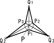
Figure 6: The “Mercedes form” for the 3Q system, where quarks are put on ${\rm Q}_{i}$ ($i$=1,2,3). The modified Y-type flux-tube length $L_{\rm\bar{Y}}$ is expressed as $L_{\rm\bar{Y}}=\frac{1}{2}\sum_{i\neq j}\overline{{\rm P}_{i}{\rm Q}_{j}}$. P denotes the Fermat point of $\triangle{\rm Q_{1}Q_{2}Q_{3}}$, and ${\rm P}_{i}$ is taken on the extended line of ${\rm Q}_{i}{\rm P}$ so as to satisfy $\overline{\rm PP}_{i}=\xi$. The “inverse Mercedes Ansatz” is defined as $\Delta E_{\rm 3Q}=K/L_{\rm\bar{Y}}+G$.

After some trials, we finally find that the “inverse Mercedes Ansatz” defined by the following functional form well reproduces the lattice QCD results for the gluonic excitation energy $\Delta E_{\rm 3Q}$ in the 3Q system:

$$\Delta E_{\rm 3Q} = \frac{K}{L_{\rm\bar{Y}}}+G,$$ (17)

$$L_{\rm\bar{Y}} \equiv {\sum_{i=1}^{3}\sqrt{x_{i}^{2}-\xi x_{i}+\xi^{2}}}\quad(x_{i}\equiv\overline{\rm PQ}_{i})$$ (18)

with three parameters, $K$, $G$ and $\xi$.

Here, we refer to $L_{\rm\bar{Y}}$ as the “modified Y-type flux-tube length”, or the “modified Y-length” simply. For $\xi=0$, $L_{\rm\bar{Y}}$ coincides with the Y-type flux-tube length $L_{\rm min}=\sum_{i=1}^{3}\overline{\rm PQ}_{i}=\sum_{i=1}^{3}x_{i}$. Note that $2L_{\rm\bar{Y}}$ expresses the total perimeter of the “Mercedes form” shown in Fig. 6, i.e.,

$$L_{\rm\bar{Y}}=\frac{1}{2}\sum_{i\neq j}\overline{{\rm P}_{i}{\rm Q}_{j}},$$ (19)

since $\overline{\rm P_{2}Q_{1}}^{2}=x_{1}^{2}+\xi^{2}-2\xi x_{1}\cos\frac{\pi}{3}=x_{1}^{2}-\xi x_{1}+\xi^{2}$ etc.

In Fig. 7, we plot the lattice QCD results of the gluonic excitation energy $\Delta E_{\rm 3Q}\equiv V^{\rm g.s.}_{\rm 3Q}-V^{\rm e.s.}_{\rm 3Q}$ against the modified Y-length $L_{\overline{\rm Y}}$ defined in Eq.(18). As a remarkable fact, $\Delta E_{\rm 3Q}$ can be plotted as a single-valued function of $L_{\rm\bar{Y}}$. In Fig. 8, we also plot $\Delta E_{\rm 3Q}\equiv V^{\rm g.s.}_{\rm 3Q}-V^{\rm e.s.}_{\rm 3Q}$ against $1/L_{\overline{\rm Y}}$, since the inverse Mercedes Ansatz corresponds to a linear arising behavior in this plot.

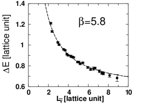
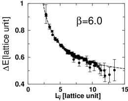
Figure 7: The lattice QCD results of the gluonic excitation energy $\Delta E_{\rm 3Q}\equiv V^{\rm g.s.}_{\rm 3Q}-V^{\rm e.s.}_{\rm 3Q}$ plotted against the modified Y-length $L_{\overline{\rm Y}}$ defined in Eq.(18). The dashed curve denotes the inverse Mercedes Ansatz with the best-fit parameters listed in Table 5.

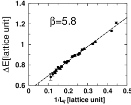
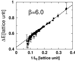
Figure 8: The lattice QCD results of the gluonic excitation energy $\Delta E_{\rm 3Q}\equiv V^{\rm g.s.}_{\rm 3Q}-V^{\rm e.s.}_{\rm 3Q}$ plotted against $1/L_{\overline{\rm Y}}$. The dashed line denotes the inverse Mercedes Ansatz with the best-fit parameters listed in Table 5.

We summarize in Table 5 the fit analysis with the inverse Mercedes Ansatz for the lattice QCD data of the gluonic excitation energy $\Delta E_{\rm 3Q}$ at each $\beta$ together with the best-fit parameter set, ($K$, $G$, $\xi$). (In Appendix, we summarize various fit analyses for $\Delta E_{\rm 3Q}$ with several trial fit functions of {$a,b,c$} or {$x_{1},x_{2},x_{3}$}.)

Table 5: The fit analysis with the “inverse Mercedes Ansatz” for the lattice QCD data of the gluonic excitation energy $\Delta E_{\rm 3Q}$ at $\beta$=5.8 and 6.0. The best-fit parameter set ($K$, $G$, $\xi$) is listed in the lattice unit. One finds $G(\beta=5.8)\simeq$ 0.77 GeV, $G(\beta=6.0)\simeq$ 0.85 GeV, $\xi(\beta=5.8)\simeq$ 0.116 fm and $\xi(\beta=6.0)\simeq$ 0.103 fm in the physical unit.

$\beta$	$K$	$G$	$\xi$	$\chi^{2}/N_{DF}$
$5.8$	1.4329(340)	0.5500(105)	0.77	41.2/(24-3)=1.96
$6.0$	1.3486(277)	0.4252( 68)	1.03	76.8/(73-3)=1.10

In Figs. 7 and 8, we have added by the dashed line the best-fit result of the inverse Mercedes Ansatz with the parameters listed in Table 5. The inverse Mercedes Ansatz seems to reproduce fairly well the lattice QCD data for the 3Q gluonic excitation energy $\Delta E_{\rm 3Q}$ at least for the short and the intermediate distances as $L_{\rm min}\leq$ 2 fm.

Note again that $\Delta E_{\rm 3Q}$ is generally a function of the three variables {$x_{1}$, $x_{2}$, $x_{3}$}. However, the inverse Mercedes Ansatz (17) depends only on $L_{\rm\bar{Y}}$, which is a single symmetric combination of {$x_{1}$,$x_{2}$,$x_{3}$}. We stress that such a simple dependence is rather nontrivial.

Now, we pay attention to the parameters $K$, $G$ and $\xi$. As the physical meaning of the parameters $\xi$ and $G$ in the inverse Mercedes Ansatz, $\xi$ plays the role of an “ultraviolet cutoff” parameter when all of $x_{i}$ are small as $x_{i}<\xi$, and the parameter $G$ seems to give an infrared value of the gluonic excitation energy. We find a relatively good scaling behavior for the parameter set $(K,G,\xi)$ in Table 5: $K(\beta=5.8)\simeq 1.43$, $K(\beta=6.0)\simeq 1.35$, $G(\beta=5.8)\simeq$ 0.77 GeV, $G(\beta=6.0)\simeq$ 0.85 GeV, $\xi(\beta=5.8)\simeq$ 0.116 fm and $\xi(\beta=6.0)\simeq$ 0.103 fm in the physical unit.

As a caution, one has to be careful for the argument on the infrared behavior of $\Delta E_{\rm 3Q}$. For, the character of the gluonic excitation mode may be changed into the stringy behavior in the infrared region, as is actually shown in the Q-$\rm\bar{Q}$ gluonic excitation mode for $r\geq 2$ fm. For the definite conclusion of the infrared behavior of $\Delta E_{\rm 3Q}$, we need to perform the lattice QCD calculation for $\Delta E_{\rm 3Q}$ with much larger lattice volume.

VI Discussion

VI.1 Physical implication of the lattice QCD results

We consider the physical meaning of the present lattice QCD result, although the precise physical interpretation of the inverse Mercedes Ansatz (17) would be rather difficult and is an open problem. Since the inverse Mercedes Ansatz is described with the modified Y-type flux-tube length $L_{\rm\bar{Y}}$, the gluonic excitation would be regarded as a global excitation of the whole Y-type flux-tube system, instead of the partial excitation of each flux-tube as ${\rm PQ}_{1}$, ${\rm PQ}_{2}$ or ${\rm PQ}_{3}$. This would exclude the quasi-fixed edge nature of the Y-type junction, as was also indicated in sectionV-A. In fact, the inverse Mercedes Ansatz indicates that the gluonic excitation in the 3Q system appears as a complicated excitation of the whole 3Q system.

As a remarkable fact on the absolute value of the gluonic excitation energy, the lowest gluonic-excitation energy $\Delta E_{\rm 3Q}$ is found to be about 1 GeV or more in the typical hadronic scale as 0.5 fm$\leq L_{\rm min}\leq$ 1.5 fm. In fact, the gluonic excitation energy $\Delta E_{\rm 3Q}$ is rather large in comparison with the low-lying excitation energy of the quark origin. (Also for the Q-${\rm\bar{Q}}$ system, a large gluonic excitation energy is reported in recent lattice studies JKM03 .) Therefore, the contribution of gluonic excitations is considered to be negligible and the dominant contribution is brought by quark dynamics such as the spin-orbit interaction for low-lying hadrons.

On the other hand, the gluonic excitation would be significant and visible in the highly-excited baryons with the excitation energy above 1 GeV. For instance, the lowest hybrid baryon CP02 , which is described as $qqqG$ in the valence picture, is expected to have a large mass of about 2 GeV. This lattice QCD result may suggest a large “constituent gluon mass” of about 1 GeV in the constituent gluon picture.

VI.2 Gluonic excitation and success of quark model

We consider the connection between QCD and the quark model in terms of the gluonic excitation TS03 ; SIT04 . While QCD is described with quarks and gluons, the simple quark model, which contains only quarks as explicit degrees of freedom, successfully describes low-lying hadrons, in spite of the absence of gluonic excitation modes and the non-relativistic treatment. As for the non-relativistic treatment, it is conjectured to be justified by a large mass generation of quarks due to dynamical chiral-symmetry breaking (DCSB). However, the absence of the gluonic excitation modes in low-lying hadron spectra has been a puzzle in the hadron physics.

On this point, we find the gluonic-excitation energy to be about 1 GeV or more, which is rather large compared with the excitation energies of the quark origin, and therefore the effect of gluonic excitations is negligible and quark degrees of freedom plays the dominant role in low-lying hadrons with the excitation energy below 1 GeV. Thus, the large gluonic-excitation energy of about 1 GeV gives the physical reason for the invisible gluonic excitation in low-lying hadron spectra, which would play the key role to the success of the quark model without gluonic excitation modes TS03 ; SIT04 .

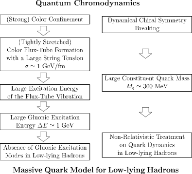
Figure 9: A possible scenario from QCD to the quark model in terms of color confinement and DCSB. DCSB leads to a large constituent quark mass of about 300 MeV, which enables the non-relativistic treatment for quark dynamics approximately. Color confinement results in the color flux-tube formation among quarks with a large string tension of $\sigma\simeq$ 1 GeV/fm. In the flux-tube picture, the gluonic excitation is described as the flux-tube vibration, and the flux-tube vibrational energy is expected to be large, reflecting the large string tension. The large gluonic-excitation energy of about 1 GeV leads to the absence of the gluonic mode in low-lying hadrons, which would play the key role to the success of the quark model without gluonic excitation modes.

In Fig. 9, by way of the flux-tube picture, we present a possible scenario from QCD to the massive quark model in terms of color confinement and DCSB SIT04 . On one hand, DCSB gives rise of a large constituent quark mass of about 300 MeV, which enables the non-relativistic treatment for quark dynamics approximately. On the other hand, color confinement results in the color flux-tube formation among quarks with a large string tension of $\sigma\simeq$ 1 GeV/fm. In the flux-tube picture, the gluonic excitation is described as the flux-tube vibration, and the flux-tube vibrational energy is expected to be large, reflecting the large string tension and the resulting short string. Due to the large gluonic-excitation energy, which is actually estimated as about 1 GeV in lattice QCD, the gluonic excitation seems invisible in low-lying hadrons. In this way, the quark model becomes successful even without explicit gluonic modes.

VII Summary and conclusion

For about 100 different patterns of spatially-fixed three-quark (3Q) systems, we have studied the excited-state 3Q potential and the gluonic excitation using SU(3) lattice QCD with $16^{3}\times 32$ at $\beta$=5.8 and 6.0 at the quenched level. We have extracted the excited-state potential $V_{\rm 3Q}^{\rm e.s.}$ together with the ground-state potential $V_{\rm 3Q}^{\rm g.s.}$ by diagonalizing the QCD Hamiltonian in the presence of three quarks, for 24 patterns of 3Q systems at $\beta=5.8$ and for 73 patters at $\beta=6.0$.

We have found that the lowest gluonic excitation energy $\Delta E_{\rm 3Q}\equiv V_{\rm 3Q}^{\rm e.s.}-V_{\rm 3Q}^{\rm g.s.}$ takes a large value of about 1 GeV at the typical hadronic scale as 0.5 fm $\leq L_{\rm min}\leq$ 1.5 fm. Therefore, we have conjectured that the “hybrid baryon” $qqqG$, which corresponds to the gluonic excitation mode, appears as the highly-excited baryon with the excitation energy of above 1 GeV.

Next, we have investigated the functional form of the gluonic excitation energy $\Delta E_{\rm 3Q}$ in terms of the 3Q location. After some trials with various functions, we have found that the lattice data of $\Delta E_{\rm 3Q}$ are relatively well reproduced by the “inverse Mercedes Ansatz”, $\Delta E_{\rm 3Q}=K/L_{\rm\bar{Y}}+G$ with the “modified Y-type flux-tube length” $L_{\rm\bar{Y}}$. This nontrivial behavior of $\Delta E_{\rm 3Q}$ seems to indicate that the gluonic-excitation mode is realized as a complicated bulk excitation of the whole Y-type flux-tube system, instead of the partial excitation of each flux-tube.

Finally, we have considered the physical consequence of the large gluonic-excitation energy, and have presented a possible scenario to give a physical reason of the success of the quark model for low-lying hadrons even without explicit gluonic modes.

These lattice QCD data of the excited-state potential would be useful for the QCD-based construction of the refined quark model, which can deal with the gluonic excitation modes in hadrons. Our results would be also helpful for the comprehension of the nature of the “QCD string”.

Appendix A Fit analyses for the gluonic excitation energy

In Appendix, we summarize various fit analyses for the gluonic excitation energy in the spatially-fixed 3Q system, $\Delta E_{\rm 3Q}\equiv V_{\rm 3Q}^{\rm e.s.}-V_{\rm 3Q}^{\rm g.s.}$, in terms of the 3Q spatial configuration. We examine various trial fit functions of {$a,b,c$} or {$x_{1},x_{2},x_{3}$} including two or three free parameters, $a_{i}$: Form 1-10 expressed by Eqs.(A1)-(A10). ({$a,b,c$} and {$x_{1},x_{2},x_{3}$} are defined in sectionV.)

Form 1 is the “inverse Mercedes Ansatz”, which is discussed in sectionV as the best fit form for the gluonic excitation energy $\Delta E_{\rm 3Q}$. Form 2 is a simplified form of Form 1. We examine Form 3-5 and Form 6-8 as the typical single-valued function of $L_{\rm min}$ and $L_{\Delta}$, respectively. As a possibility, the gluonic excitation energy $\Delta E_{\rm 3Q}$ may be controlled by the “typical length” of the static 3Q system, and hence we examine also Form 9 and Form 10, regarding $\max(x_{1}+x_{2},x_{2}+x_{3},x_{3}+x_{1})$ and $\max(a,b,c)$ as the typical length of the Y-type flux-tube system.

For each of Form 1-10, we show $\chi^{2}/N_{\rm DF}$ as the fit result for the lattice data of $\Delta E_{\rm 3Q}$ together with the best-fit parameters in Tables 6 and 7 at $\beta$=5.8 and 6.0, respectively.

As a result, Form 1, the “inverse Mercedes Ansatz”, is found to be the best fit function for $\Delta E_{\rm 3Q}$, which reproduces the lattice data of $\Delta E_{\rm 3Q}$ with the smallest $\chi^{2}/N_{\rm DF}\sim 1$.

Table 6: The best-fit analysis for the lattice QCD data of the gluonic excitation energy $\Delta E_{\rm 3Q}$ at $\beta$=5.8 with various trial fit functions. For each form, the best-fit parameters $a_{i}$ are listed with the $\chi^{2}/N_{\rm DF}$.

Form	$a_{1}$	$a_{2}$	$a_{3}$	$\chi^{2}/N_{\rm DF}$
(A1)	1.4329(340)	0.5500(105)	0.77	1.96
(A2)	2.0996(501)	0.4936(117)	0.55	2.16
(A3)	2.6676(3674)	1.7127(3568)	0.4734(339)	3.44
(A4)	-0.2017(2759)	0.3210(293)	1.4428(928)	3.27
(A5)	0.3818(827)	1.4193(1612)	0.1044(1879)	3.29
(A6)	5.1692(7427)	3.4586(6932)	0.4515(369)	2.18
(A7)	-0.0067(5676)	0.3417(334)	1.8386(1740)	2.02
(A8)	0.3269(830)	1.8641(1922)	-0.0411(2578)	2.02
(A9)	0.9341(213)	0.6304(89)	—	11.71
(A10)	0.8065(183)	0.6352(87)	—	12.84

Table 7: The best-fit analysis for the lattice data of $\Delta E_{\rm 3Q}$ at $\beta$=6.0 with various trial fit functions.

Form	$a_{1}$	$a_{2}$	$a_{3}$	$\chi^{2}/N_{\rm DF}$
(A1)	1.3486(277)	0.4252(68)	1.03	1.10
(A2)	1.9810(410)	0.3860(73)	1.01	1.52
(A3)	2.3757(2175)	2.0816(3065)	0.3794(146)	2.59
(A4)	-0.5066(2125)	0.2871(164)	1.0987(459)	2.53
(A5)	0.4284(559)	1.0722(495)	0.1760(694)	2.54
(A6)	4.6197(4238)	4.2849(5709)	0.3644(156)	1.57
(A7)	-0.3829(4184)	0.3065(180)	1.3764(780)	1.54
(A8)	0.3659(538)	1.3968(512)	0.0862(919)	1.54
(A9)	0.82575(164)	0.4846(63)	—	8.67
(A10)	0.7164(143)	0.4864(63)	—	9.31

• Form 1 (The inverse Mercedes Ansatz)

  $$\Delta E_{\rm 3Q}=\frac{a_{1}}{L_{\rm\overline{Y}}}+a_{2}=\frac{a_{1}}{\sum_{i}\sqrt{x_{i}^{2}-x_{i}a_{3}+a_{3}^{2}}}+a_{2}$$ (20)

• Form 2

  $$\Delta E_{\rm 3Q} = \frac{a_{1}}{\sum_{i}\sqrt{x_{i}^{2}+a_{3}^{2}}}+a_{2}$$ (21)

• Form 3

  $$\Delta E_{\rm 3Q}=\frac{a_{1}}{L_{\rm min}+a_{2}}+a_{3}$$ (22)

• Form 4

  $$\Delta E_{\rm 3Q}=\frac{a_{3}}{(L_{\rm min}+a_{1})^{a_{2}}}$$ (23)

• Form 5

  $$\Delta E_{\rm 3Q}=\frac{a_{2}}{{L_{\rm min}}^{a_{1}}}+a_{3}$$ (24)

• Form 6

  $$\Delta E_{\rm 3Q}=\frac{a_{1}}{L_{\Delta}+a_{2}}+a_{3}$$ (25)

• Form 7

  $$\Delta E_{\rm 3Q}=\frac{a_{3}}{(L_{\Delta}+a_{1})^{a_{2}}}$$ (26)

• Form 8

  $$\Delta E_{\rm 3Q}=\frac{a_{2}}{{L_{\Delta}}^{a_{1}}}+a_{3}$$ (27)

• Form 9

  $$\Delta E_{\rm 3Q}=\frac{a_{1}}{\max(x_{1}+x_{2},x_{2}+x_{3},x_{3}+x_{1})}+a_{2}$$ (28)

• Form 10

  $$\Delta E_{\rm 3Q}=\frac{a_{1}}{\max(a,b,c)}+a_{2}$$ (29)

References

- (1) Y. Nambu, in Preludes in Theoretical Physics, in honor of V.F. Weisskopf (North-Holland, Amsterdam, 1966); H. Fritzsch, M. Gell-Mann, and H. Leutwyler, Phys. Lett. B47, 365 (1973); D.J. Gross and F. Wilczek, Phys. Rev. Lett. 30, 1343 (1973); H.D. Politzer, Phys. Rev. Lett. 30, 1346 (1973); S. Weinberg, Phys. Rev. Lett. 31, 494 (1973).
- (2) For instance, CP-PACS Collaboration (A. Ali Khan et al.), Phys. Rev. D65, 054505 (2002); Erratum-ibid. D67, 059901 (2003).
- (3) For recent review articles, J.B. Kogut, Nucl. Phys. B (Proc. Suppl.) 119, 210 (2003); S.D. Katz, Nucl. Phys. B (Proc. Suppl.) 129, 60 (2004).
- (4) Y. Nambu, in Symmetries and Quark Models (Wayne State University, 1969).
- (5) Y. Nambu, Lecture Notes at the Copenhagen Symposium (1970).
- (6) G. Veneziano, Nuovo Cim. A57, 190 (1968).
- (7) Y. Nambu, Phys. Rev. D10, 4262 (1974).
- (8) J. Kogut and L. Susskind, Phys. Rev. D11, 395 (1975).
- (9) J. Polchinski, String Theory, Cambridge Monographs on Mathematical Physics, (Cambridge University Press, 1998) p.1.
- (10) R. Hagedorn, Nuovo Cim. Suppl. 3, 147 (1965).
- (11) A. Patel, Nucl. Phys. B243, 411 (1984); Phys. Lett. B139, 394 (1984).
- (12) A. Casher, H. Neuberger, and S. Nussinov, Phys. Rev. D20, 179 (1979).
- (13) S. Capstick and N. Isgur, Phys. Rev. D34, 2809 (1986).
- (14) H. Suganuma, S. Sasaki, and H. Toki, Nucl. Phys. B435, 207 (1995).
- (15) T.T. Takahashi and H. Suganuma, Phys. Rev. Lett. 90, 182001 (2003).
- (16) H. Suganuma, H. Ichie, and T.T. Takahashi, in Color Confinement and Hadrons in Quantum Chromodynamics edited by H. Suganuma, N. Ishii, M. Oka, H. Enyo, T. Hatuda, T. Kunihiro, and K. Yazaki (World Scientific, Singapore, 2004) p.249; T.T. Takahashi, H. Suganuma, H. Ichie, H. Matsufuru, and Y. Nemoto, Nucl. Phys. A721, 926 (2003); H. Suganuma, T.T. Takahashi, and H. Ichie, Nucl. Phys. A737, S27 (2004).
- (17) K.J. Juge, J. Kuti, and C.J. Morningstar, Phys. Rev. Lett. 90, 161601 (2003); Nucl. Phys. B (Proc. Suppl.) 63, 326 (1998).
- (18) J.F. Donoghue, E. Golowich, and B.R. Holstein, Dynamics of the Standard Model, Cambridge Monographs on Particle Physics, Nuclear Physics and Cosmology, (Cambridge University Press, 1992).
- (19) T.T. Takahashi, H. Matsufuru, Y. Nemoto, and H. Suganuma, Proc. of the Int. Symp. on Dynamics of Gauge Fields, Tokyo, 1999, edited by A. Chodos, N. Kitazawa, H. Minakata, and C.M. Sommerfield (Universal Academy Press, 2000) p.179; H. Suganuma, Y. Nemoto, H. Matsufuru, and T.T. Takahashi, Nucl. Phys. A680, 159 (2000).
- (20) T.T. Takahashi, H. Matsufuru, Y. Nemoto, and H. Suganuma, Phys. Rev. Lett. 86, 18 (2001).
- (21) T.T. Takahashi, H. Suganuma, Y. Nemoto, and H. Matsufuru, Phys. Rev. D65, 114509 (2002).
- (22) M. Creutz, Phys. Rev. Lett. 43, 553 (1979), Erratum-ibid. 43, 890 (1979); Phys. Rev. D21, 2308 (1980).
- (23) G.S. Bali and K. Schilling, Phys. Rev. D46, 2636 (1992).
- (24) For a review article, G.S. Bali, Phys. Rept. 343, 1 (2001) and references therein.
- (25) M. Lüscher and P. Weisz, JHEP 0109, 010 (2001).
- (26) R. Sommer and J. Wosiek, Phys. Lett 149B, 497 (1984); Nucl. Phys. B267, 531 (1986).
- (27) J. Kamesberger, G. Eder, M.E. Fabar, H. Leeb, and H. Markum, in Few-Body Problems in Particle, Nuclear, Atomic, and Molecular Physics, Proc. of XIth European Conference on Few-Body Physics, Fontevraud, 1987, edited by J.-L. Ballot and M. Fabre de la Ripelle (Springer-Verlag, Vienna, 1987), p. 529.
- (28) H.B. Thacker, E. Eichten, and J.C. Sexton, Nucl. Phys. B (Proc. Suppl.) 4, 234 (1988).
- (29) M. Fabre de la Ripelle and Yu. A. Simonov, Ann. Phys. 212, 235 (1991).
- (30) N. Brambilla, G.M. Prosperi, and A. Vairo, Phys. Lett. B362, 113 (1995).
- (31) F. Okiharu, H. Suganuma, and T.T. Takahashi, “First study for the pentaquark potential in SU(3) lattice QCD”, hep-lat/0407001; H. Suganuma, T.T. Takahashi, F. Okiharu, and H. Ichie, in QCD Down Under, Adelaide, March 2004, Nucl. Phys. B (Proc. Suppl.) in press.
- (32) C. Alexandrou, P. de Forcrand, and A. Tsapalis, Phys. Rev. D65, 054503 (2002).
- (33) O. Jahn and P. de Forcrand, Nucl. Phys. B (Proc. Suppl.) 129, 700 (2004).
- (34) J.M. Cornwall, Phys. Rev. D54, 6527 (1996).
- (35) J.M. Cornwall, Phys. Rev. D69, 065013 (2004).
- (36) D.S. Kuzmenko and Yu.A. Simonov, Phys. Atom. Nucl. 66, 950 (2003).
- (37) H. Ichie, V. Bornyakov, T. Streuer, and G. Schierholz, Nucl. Phys. A721, 899 (2003); Nucl. Phys. B (Proc. Suppl.) 119, 751 (2003).
- (38) APE Collaboration, M. Albanese et al., Phys. Lett. B192, 163 (1987).
- (39) M. Lüscher and U. Wolff, Nucl. Phys. B339, 222 (1990).
- (40) S. Perantonis and C. Michael, Nucl. Phys. B347, 854 (1990).
- (41) S. Capstick and P.R. Page, Phys. Rev. C66, 065204 (2002).