Topological susceptibility for the SU(3) Yang–Mills theory

Abstract

We present the results of a computation of the topological susceptibility in the SU(3) Yang–Mills theory performed by employing the expression of the topological charge density operator suggested by Neuberger’s fermions. In the continuum limit we find $r_{0}^{4}\chi=0.059(3)$, which corresponds to $\chi=(191\pm 5\,\mathrm{MeV})^{4}$ if $F_{K}$ is used to set the scale. Our result supports the Witten–Veneziano explanation for the large mass of the $\eta^{\prime}$.

1 Introduction

The topological susceptibility in the Yang–Mills (YM) gauge theory can be formally defined in Euclidean space-time as

$$\chi=\int d^{4}x\>\langle q(x)q(0)\rangle\;,$$ (1)

where the topological charge density $q(x)$ is

$$q(x)=-\frac{1}{32\pi^{2}}\epsilon_{\mu\nu\rho\sigma}\mathrm{Tr}\Big{[}F_{\mu\nu}(x)F_{\rho\sigma}(x)\Big{]}\;.$$ (2)

Besides its interest within the pure gauge theory, $\chi$ plays a crucial rôle in the QCD-based explanation of the large mass of the $\eta^{\prime}$ meson proposed by Witten and Veneziano (WV) [1, 2]. The WV mechanism predicts that, at leading order in $N_{\mathrm{f}}/N_{\mathrm{c}}$, the contribution due to the anomaly to the mass of the $U_{\mathrm{A}}(1)$ particle is given by [1, 2, 3, 4]

$$\frac{F_{\pi}^{2}m^{2}_{\eta^{\prime}}}{2N_{\mathrm{f}}}=\chi\,,$$ (3)

where $F_{\pi}$ is the pion decay constant. The discovery of a fermion operator [5] that satisfies the Ginsparg–Wilson (GW) relation [6] triggered a breakthrough in the understanding of the topological properties of the YM vacuum [7, 8, 4, 9, 10], and made it possible to give a precise and unambiguous implementation of the WV formula [4]. Indeed the naive lattice definition of the topological susceptibility has a finite continuum limit, which is universal [10], if the topological charge density, defined as suggested by GW fermions, is employed [4, 9, 10]. This yields the suggestive formula

$$\chi=\lim_{\begin{array}[]{c}a\rightarrow 0\\ V\rightarrow\infty\end{array}}\frac{\langle Q^{2}\rangle}{V}$$ (4)

with $Q\equiv\sum_{x}q(x)=n_{+}-n_{-}$ being the topological charge, $V$ the volume, and $n_{+}$ ($n_{-}$) the number of zero modes of $D$ with positive (negative) chirality in a given background. Using new simulation algorithms [11], it is now possible to investigate the WV scenario from first principles for the first time. More precisely, the aim of the work presented here, and fully described in [12], is to achieve an accurate and reliable determination of $\chi$ in the continuum limit, which in turn allows a verification of the WV mechanism for the $\eta^{\prime}$ mass. Several exploratory computations have already studied the susceptibility employing the GW definition of the topological charge [13, 14, 15, 16, 17, 18, 19].

Figure 1: Comparison with other computations.

2 Lattice computation

The ensembles of gauge configurations are generated with the standard Wilson action and periodic boundary conditions, using a combination of heat-bath and over-relaxation updates. More details on the generation of the gauge configurations can be found in Refs. [18, 19]. Table 1 shows the list of simulated lattices, where the bare coupling constant $\beta=6/g_{0}^{2}$, the linear size $L/a$ in each direction and the number of independent configurations are reported for each lattice. The topological charge density is defined as

$$q(x)=-\frac{\bar{a}}{2}\,\mathrm{Tr}\Big{[}\gamma_{5}D(x,x)\Big{]},$$ (5)

with $D$ being the massless Neuberger–Dirac operator [5], and $s$ an adjustable parameter in the range $|s|<1$. For a given gauge configuration, the topological charge is computed by counting the number of zero modes of $D$ (the interested reader should refer to [12] for more details). As $s$ is varied, $D$ defines a one-parameter family of fermion discretizations, which correspond to the same continuum theory but with different discretization errors at finite lattice spacing. Our computation includes data sets computed for $s=0.4$ and $s=0.0$. A comparison with results previously obtained with various implementation of the Neuberger’s operator is shown in Fig. 1.

lat	$\beta$	$L/a$	$N_{\mathrm{conf}}$	$\langle Q^{2}\rangle$	$r_{0}^{4}\chi$
${\rm A}_{1}$	$6.0$	$12$	$2452$	$1.633(48)$	$0.0654(22)$
${\rm A}_{2}$	$6.1791$	$16$	$1138$	$1.589(76)$	$0.0629(32)$
${\rm A}_{3}$	$5.8989$	$10$	$1460$	$1.737(72)$	$0.0696(30)$
${\rm A}_{4}$	$6.0938$	$14$	$1405$	$1.535(63)$	$0.0615(27)$
${\rm B}_{0}$	$5.8458$	$12$	$2918$	$5.61(16)$	$0.0715(22)$
${\rm B}_{1}$	$6.0$	$16$	$1001$	$5.58(28)$	$0.0707(37)$
${\rm B}_{2}$	$6.1366$	$20$	$963$	$4.81(24)$	$0.0604(32)$
${\rm B}_{3}$	$5.9249$	$14$	$1284$	$5.59(24)$	$0.0708(33)$
${\rm C}_{0}$	$5.8784$	$16$	$1109$	$15.02(72)$	$0.0784(39)$
${\rm C}_{1}$	$6.0$	$20$	$931$	$12.76(95)$	$0.0662(50)$
${\rm D}$	$6.0$	$14$	$1577$	$3.01(12)$	$0.0651(27)$
${\rm E}$	$5.9$	$12$	$1349$	$2.79(12)$	$0.0543(24)$
${\rm F}$	$5.95$	$12$	$1291$	$1.955(79)$	$0.0551(24)$
${\rm G}$	$6.0$	$12$	$3586$	$1.489(37)$	$0.0596(18)$
${\rm H}$	$6.1$	$16$	$962$	$2.45(13)$	$0.0599(33)$
${\rm J}$	$6.2$	$18$	$1721$	$2.114(76)$	$0.0591(24)$

Table 1: Simulation parameters and results. For lattices ${\rm A}_{1}$–${\rm D}$ and ${\rm E}$–${\rm J}$, $s=0.4$ and $s=0.0$ respectively.

The systematic uncertainties stem from finite-volume effects and from the extrapolation needed to reach the continuum limit. The pure gauge theory has a mass gap, and therefore the topological susceptibility approaches the infinite-volume limit exponentially fast with $L$. Since the mass of the lightest glueball is around 1.5 GeV, finite-volume effects are expected to be far below our statistical errors as soon as $L\geq 1$ fm. In order to further verify that no sizeable finite-volume effects are present in our data, we simulated four lattices at $\beta=6.0$ but with different linear sizes. The results obtained for $\chi$, reported in Table 1, show no dependence on $L$ within our statistical errors.

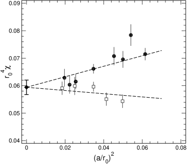
Figure 2: Continuum extrapolation of the adimensional product $r_{0}^{4}\chi$. The $s=0.0$ and $s=0.4$ data sets are represented by black circles and white squares respectively. The dashed lines represent the results of the combined fit described in the text. The filled diamond at $a=0$ is the extrapolated value in the continuum limit.

At finite lattice spacing, $\chi$ is affected by discretization effects starting at $O(a^{2})$, which are not universal, and, in our case, depend on the value of $s$ chosen to define the Neuberger operator. The values of the adimensional quantity $r_{0}^{4}\chi$ that we obtain, where $r_{0}/a$ is taken from [20], are reported in Table 1. Data, displayed in Fig. 2 as a function of $a^{2}/r_{0}^{2}$, show sizeable $O(a^{2})$ effects for both the $s=0.4$ and $s=0.0$ samples. For $\beta\leq 6.0$, the difference between the two discretizations is statistically significant. A detailed data analysis indicate a linear dependence in $a^{2}$ of our results within our statistical errors [12].

3 Conclusions

A robust estimate of $\chi$ in the continuum limit can be obtained by performing a combined linear fit of the data. This fit gives a very good value of $\chi^{2}_{\mathrm{dof}}$ when all sets are included, and is very stable if some points at larger values of $a^{2}/r_{0}^{2}$ are removed. In particular a combined fit of all points with $a^{2}/r_{0}^{2}<0.05$ gives $c_{0}=0.059(3)$ with $\chi^{2}_{\mathrm{dof}}\approx 0.73$. Since $r_{0}$ is not directly accessible to experiments, we express our result in physical units by using the lattice determination of $r_{0}F_{K}=0.4146(94)$ in the quenched theory [21] and we obtain

$$\chi=(191\pm 5\,\mathrm{MeV})^{4}\,,$$ (6)

which has to be compared with [2]

$$\frac{F_{\pi}^{2}}{6}\Big{(}m^{2}_{\eta}+m^{2}_{\eta^{\prime}}-2m^{2}_{K}\Big{)}\Big{|}_{\mathrm{exp}}\simeq(180\,\mathrm{MeV})^{4}\;.$$ (7)

Notice that Eq. (3) being only valid at the leading order in a $N_{\mathrm{f}}/N_{\mathrm{c}}$ expansion, the ambiguity in the conversion to physical units in the pure gauge theory is of the same order as the neglected terms. Our result supports the Witten–Veneziano mechanism for explaining the large $\eta^{\prime}$ mass. A measurement of the connected expectation values $\langle Q^{2n}\rangle_{c}$ with the methods presented here would provide interesting informations about the dependence of the free energy density on the $\theta$ angle, or equivalently on the probability distribution of the topological charge $P_{Q}$, putting on solid ground the results presented in Ref. [22]. Unfortunately much higher statistics are required in order to highlight the deviations from a Gaussian distribution; higher momenta of the topological charge distribution measured on our data are all compatible with zero within large statistical errors.

References

- [1] E. Witten, Nucl. Phys. B156 (1979) 269.
- [2] G. Veneziano, Nucl. Phys. B159 (1979) 213.
- [3] E. Seiler, I.O. Stamatescu, MPI-PAE/PTh 10/87.
- [4] L. Giusti et al., Nucl. Phys. B628 (2002) 234.
- [5] H. Neuberger, Phys. Rev. D57 (1998) 5417.
- [6] P.H. Ginsparg, K.G. Wilson, Phys. Rev. D25 (1982) 2649.
- [7] P. Hasenfratz, V. Laliena, F. Niedermayer, Phys. Lett. B427 (1998) 125.
- [8] M. Luscher, Phys. Lett. B428 (1998) 342.
- [9] L. Giusti et al., Phys. Lett. B587 (2004) 157.
- [10] M. Lüscher, hep-th/0404034.
- [11] L. Giusti et al., Comput. Phys. Commun. 153 (2003) 31.
- [12] L. Del Debbio, L. Giusti, C. Pica, hep-th/0407052.
- [13] R.G. Edwards, U.M. Heller, R. Narayanan, Phys. Rev. D59 (1999) 094510.
- [14] T. DeGrand, U.M. Heller (MILC), Phys. Rev. D65 (2002) 114501.
- [15] C. Gattringer, R. Hoffmann, S. Schaefer, Phys. Lett. B535 (2002) 358.
- [16] P. Hasenfratz et al., Nucl. Phys. B643 (2002) 280.
- [17] T.W. Chiu, T.H. Hsieh, Nucl. Phys. B673 (2003) 217.
- [18] L. Giusti et al., JHEP 11 (2003) 023.
- [19] L. Del Debbio, C. Pica, JHEP 02 (2004) 003.
- [20] M. Guagnelli, R. Sommer, H. Wittig (ALPHA), Nucl. Phys. B535 (1998) 389.
- [21] J. Garden et al. (ALPHA), Nucl. Phys. B571 (2000) 237.
- [22] L. Del Debbio, H. Panagopoulos and E. Vicari, JHEP 0208 (2002) 044.