The charm quark mass with dynamical fermions

Abstract

We compute the charm quark mass in lattice QCD and compare different formulations of the heavy quark, and quenched data to that with dynamical sea quarks. We take the continuum limit of the quenched data by extrapolating from three different lattice spacings, and compare to data with two flavours of dynamical sea quarks with a mass around the strange at the coarsest lattice spacing. Both the FNAL and ALPHA formalism are used. We find the different heavy quark formulations have the same continuum limit in the quenched approximation, and limited evidence that this approximation overestimates the charm quark mass.

1 INTRODUCTION

The charm quark mass is a relatively unknown quantity, yet this is a quantity which is readily calculable on the lattice. The Particle Data Group [1] quote

$$1.0<\overline{m}_{\rm charm}^{\overline{MS}}(\overline{m}_{\rm charm})<1.4\ {\rm GeV}$$ (1)

Most lattice calculations to date have been done in the quenched approximation. In this work we compare the results of the quenched continuum limit from three lattice spacings, using different heavy quark formulations to results with two flavours of dynamical fermions with a mass around that of the strange quark. An idea of how heavy the sea quarks are can be seen by comparing the value of $m_{PS}/m_{V}\sim 0.7$ to the physical value of $m_{\pi}/m_{\rho}\sim 0.18$. Preliminary results were presented at the previous lattice conference [2] and results for the $D_{s}$ spectrum were presented in [3].

2 DETAILS OF THE CALCULATION

We used the Wilson plaquette gauge action and the Sheikholeslami-Wohlert action with a non-perturbative (NP) determination of the coefficient $c_{SW}$. At each lattice spacing we computed different definitions of the quark mass, for different values of the hopping parameter. We fixed the charm mass using the $m_{Ds}$ pseudoscalar meson. The details of the matching between the quenched and dynamical ensembles can be found in [4]. The details of the ensembles are shown in Table 1. Throughout this work the scale is set by $r_{0}=0.5$ fm.

Table 1: Ensembles of gauge configurations. $\kappa_{\rm sea}=0$ denotes a quenched ensemble. $N_{G}$ denote the number of configurations.

$(\beta,\kappa_{\rm sea})$	Volume	$a^{-1}$ (GeV)	$N_{G}$
$(6.2,0)$	$24^{3}\times 48$	$2.93$	$216$
$(6.0,0)$	$16^{3}\times 48$	$2.12$	$302$
$(5.93,0)$	$16^{3}\times 32$	$1.86$	$278$
$(5.2,0.1350)$	$16^{3}\times 32$	$1.88$	$395$

2.1 Definitions of quark mass

The quark mass can be defined in a number of ways. It can be defined from the quark coupling, $\kappa$,

$$am_{0}=\frac{1}{2}\left(\frac{1}{\kappa}-\frac{1}{\kappa_{\rm crit}}\right)$$ (2)

where $\kappa_{\rm crit}$ is the value of the hopping parameter which corresponds to zero quark mass. The renormalised quark mass, in the mass independent scheme (ALPHA), is then

$$am_{V}=Z_{M}\left(1+b_{m}am_{0}\right)am_{0}$$ (3)

Another quark mass can be defined from the Axial Ward identity, and correlation functions

$$am_{ij}=\frac{\sum_{\vec{x}}\langle\partial^{4}A^{4}_{ij}(x)P_{ij}(0)\rangle}{2\sum_{\vec{x}}\langle P_{ij}(x)P_{ij}(0)\rangle}$$ (4)

where $A$ is the improved Axial quark current, $P$ the Pseudoscalar density, ans $i$ and $j$ label quark flavour. The subscripts $i,j$ denote different quark flavours. For heavy-light correlation functions, the renormalised quark mass is

$$am_{A} = \frac{Z_{A}}{Z_{P}}\left[2\left(1+(b_{A}-b_{P})\frac{1}{2}a\overline{m}_{0}\right)\right.$$

$$\left.am_{HL}-\left(1+(b_{A}-b_{P})am^{L}_{0}\right)am_{LL}\right]$$

where $\overline{m}_{0}=\frac{1}{2}(m_{0}^{H}+m_{0}^{L})$.

The values of all the improvement and renormalisation coefficients have been determined to one loop in tadpole improved perturbation theory [5] in the $\overline{MS}$ scheme, as the NP determinations are not available for the coarsest lattice spacings.

We also use the effective field theory formalism known as the FNAL method. This presumes the dominance of ${\mathcal{O}}(am)^{n}$ lattice artefacts over ${\mathcal{O}}(ap)^{2}$. This can be seen by considering the distortion of the dispersion relation by the lattice,

$$E^{2}=M_{1}^{2}+\frac{M_{1}}{M_{2}}p^{2}+O(p^{4})$$ (6)

where $M_{1}$ is the rest mass and $M_{2}$ is the kinetic mass, defined by

$$\frac{1}{M_{2}}=\frac{\partial^{2}E}{\partial p_{k}^{2}}\mid_{p=0}$$ (7)

It is the kinetic mass which is important for the dynamics of states containing a heavy quark. The definitions of quark mass have $am_{0}$ corrections to all orders in $a$, to a particular order in $\alpha_{S}$. At tree-level the quark mass is,

$$am_{1}=\log(1+am_{0})$$ (8)

A perturbative definition of the kinetic mass is give by

$$am_{2}(am_{1})=\frac{e^{am_{1}}\sinh(am_{1})}{1+\sinh(am_{1})}$$ (9)

These quark masses can be used to determine the kinetic hadron mass,

$$aM_{2}^{PT}=aM_{1}+(am_{2}-am_{1})$$ (10)

The tree-level quark masses give a poor estimate of the kinetic mass shift. However, using the one-loop masses, the perturbative $M_{2}$ tracks the NP $M_{2}$ from the dispersion relation, without the increase in statistical errors coming from non-zero momentum states. The one-loop expressions relating the lattice quark mass and the pole quark mass are,

$$m_{1}^{(1)}=m_{1}^{(0)}+g^{2}Z_{m_{1}}^{(1)}\tanh m_{1}^{(0)}$$ (11)

$$m_{2}^{(1)}=m_{2}^{(0)}(m_{1}^{(0)}+g^{2}m_{1}^{(0)})(1+g^{2}Z_{m_{2}}^{(1)})$$ (12)

where the $Z$ functions are given in [7]. We now refer to $m^{(1)}_{1,2}$ as $m_{1,2}$ for brevity. These pole quark masses are then matched to the $\overline{MS}$ mass using the one-loop expression from [8].

We interpolate each of the four quark masses $\{m_{A},m_{V},m_{1},m_{2}\}$ from equations (3),(2.1),(11) and (12) against the pseudoscalar heavy-light meson mass, where the light quark mass has been interpolated to the strange quark mass. We denote this $M_{Hs}$. All the quark masses have corrections which scale with the quark mass, but the inverse hadron mass scales with quark mass, so it is unclear whether to plot $am_{Q}$ vs. $1/M_{Hs}$ or vs. $M_{Hs}$. We do the latter as we are interpolating in a finite range of $am_{Q}$, where a polynomial in $am_{Q}$ can be expanded in terms of $1/am_{Q}$. The heavy quark interpolation for $m_{A}$ on the matched ensembles is shown in figure 1. For ensembles with four different heavy quarks ($\beta=\{6.2,6.0\}$) we use a quadratic function, for ensembles with three ($\beta=\{5.93.5.2\}$ we use a linear function.

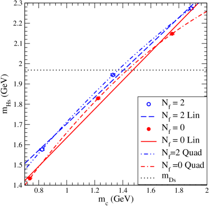
Figure 1: The hadron mass versus the $m_{A}$ quark mass for the ensembles $(\beta=5.2,\kappa=0.1350)$ and $\beta=5.93,\kappa=0)$.

The resulting charm mass is in the $\overline{MS}$ scheme at the scale of the lattice spacing. We evolve this mass using the renormalisation group equation evaluated in a package called RunDec [9] to the scale invariant mass. We can then compare the different quark masses and take the continuum limit of the quenched data.

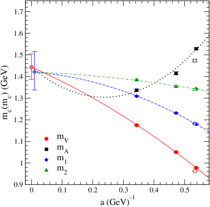
Figure 2: The quenched continuum limit of the scale invariant charm quark mass. The closed (open) symbols show the quenched (dynamical fermion) data. The shaded circle is the continuum limit of the ALPHA masses and the diamond (offset for clarity) the FNAL masses.

2.2 Comparing quark masses

Shown in figure 2 is the quenched continuum limit. The leading lattice artefacts are ${\mathcal{O}}(\alpha_{S}am)$, ${\mathcal{O}}(\alpha_{S}a)$ and ${\mathcal{O}}(a^{2})$. For the masses $m_{A}$ and $m_{V}$ these are clearly large and a linear extrapolation is not possible. However, they should have a common continuum limit, as demonstrated by Rolf and Sint [6]. We enforce the common continuum limit and perform a simultaneous quadratic fit to both masses. Within large errors this is consistent with the result from Rolf and Sint. We perform a similar fit to the FNAL masses. The two methods agree in the continuum limit.

The open symbols show the dynamical data. The dynamical ALPHA masses are lower than the quenched data. However, this is not repeated for the masses $m_{1}$ and $m_{2}$, and the sea quark mass is still rather heavy. Moreover, the dynamical and quenched data could be effected by different lattice artefacts.

Our analysis has larger statistical and systematic uncertainties than the quenched result of Rolf and Sint, and other calculations. However, we have demonstrated that the charm mass in the FNAL and ALPHA schemes has the same continuum limit. We have also found evidence which suggests the mass of the charm quark is too high in the quenched approximation at fixed lattice spacing, even though the mass of the sea quarks in the dynamical calculation is still rather heavy.

References

- [1] K. Hagiwara et al., Phys. Rev. D66, 010001 (2002).
- [2] A. Dougall, C. M. Maynard, and C. McNeile, Nucl. Phys. Proc. Suppl. 129, 170 (2004).
- [3] A. Dougall, R. D. Kenway, C. M. Maynard, and C. McNeile, Phys. Lett. B569, 41 (2003).
- [4] C. R. Allton et al., Phys. Rev. D60, 034507 (1999).
- [5] T. Bhattacharya, R. Gupta, W.-J. Lee, and S. R. Sharpe, Phys. Rev. D63, 074505 (2001).
- [6] J. Rolf and S. Sint, JHEP 12, 007 (2002).
- [7] B. P. G. Mertens, A. S. Kronfeld, and A. X. El-Khadra, Phys. Rev. D58, 034505 (1998).
- [8] N. Gray, D. J. Broadhurst, W. Grafe, and K. Schilcher, Z. Phys. C48, 673 (1990).
- [9] K. G. Chetyrkin, J. H. Kuhn, and M. Steinhauser, Comput. Phys. Commun. 133, 43 (2000).