Excited $B$ mesons from the lattice

Abstract

The energies of different angular momentum states of a heavy-light meson were measured on a lattice in [1]. We have now repeated this study using several different lattices, quenched and unquenched, that have different physical lattice sizes, clover coefficients and quark–gluon couplings. The heavy quark is taken to be infinitely heavy, whereas the light quark mass is approximately that of the strange quark. By interpolating and extrapolating in the light quark mass we can thus compare the lattice results with $B$ and $B_{s}$ meson experiments. Most interesting is the lowest P-wave $B_{s}$ state, since it is possible that it lies below the $BK$ threshold and hence is very narrow. Unfortunately, there are no experimental results on P-wave $B$ or $B_{s}$ mesons available at present.

In addition to the energy spectrum, we measured earlier also vector (charge) and scalar (matter) radial distributions of the light quark in the S-wave states of a heavy-light meson on a lattice [2]. Now we are extending the study of radial distributions to P-wave states.

1 Energies

The basic quantity for evaluating the energies of heavy-light mesons is the 2-point correlation function — see Fig. 1 a). It is defined as

$$C_{2}(T)=\langle P_{t}\Gamma G_{q}(\mathbf{x},t+T,t)\\ \cdot P_{t+T}\Gamma^{{\dagger}}U^{Q}(\mathbf{x},t,t+T)\rangle,$$ (1)

where $U^{Q}(\mathbf{x},t,T)$ is the heavy (infinite mass)-quark propagator and $G_{q}(\mathbf{x},t+T,t)$ the light anti-quark propagator. $P_{t}$ is a linear combination of products of gauge links at time $t$ along paths $P$ and $\Gamma$ defines the spin structure of the operator. The $\langle...\rangle$ means the average over the whole lattice. The energies are then extracted by fitting the $C_{2}$ with a sum of exponentials,

$$C_{2}(T)\approx\sum_{i=1}^{N_{\textrm{max}}}c_{i}\mathrm{e}^{-m_{i}T},$$ (2)

where $N_{\textrm{max}}=2\textrm{ -- }4$, $T\leq 10$.

Figure 1: a) Two-point correlation function $C_{2}$; b) Three-point correlation function $C_{3}$.

a)	b)

Table 1: Lattice parameters.

	$\beta$	$C_{\textrm{SW}}$	$\kappa$
Q3	5.7	1.57	0.14077
DF2	5.2	1.76	0.1395
DF3	5.2	2.0171	0.1350
	$a$ [fm]	$m_{q}/m_{s}$	$r_{0}m_{\pi}$
Q3	0.179(9)	0.83	1.555(6)
DF2	0.152(8)	1.28	1.94(3)
DF3	0.110(6)	1.12	1.93(3)

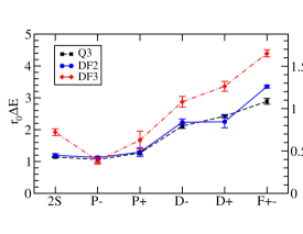
Figure 2: The energy spectrum for different angular momentum states. Here L$+$($-$) means that the light quark spin couples to angular momentum L giving the total $j=L\pm 1/2$. 2S is the first radially excited $L=0$ state. The spectrum was measured using different lattices: Q3 (a $16^{3}\times 24$ quenched lattice, [1]) and DF2, DF3 ($16^{3}\times 24$ and $16^{3}\times 32$ lattices respectively, dynamical fermions, [3]). Here $r_{0}=0.525(25)$ fm. Lattice parameters are given in Table 1. Note that the spectrum shows an approximately linear rise in excitation energy with L.

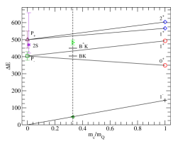
Figure 3: Interpolation from infinite mass to $m_{Q}=m_{b}$. The results at $m_{Q}=m_{c}$ are from experiments. Note that the lowest $B_{s}$ P-wave state lies below the $BK$ threshold and should be very narrow.

From some theoretical considerations [4] it is expected that, for higher angular momentum states, the multiplets should be inverted compared with the Coulomb spectrum, i.e. L$-$ should lie higher than L$+$ (see caption of Fig. 2 for notation). Experimentally this inversion is not seen for P-waves, and now the lattice measurements show that there is no inversion in the D-wave states either. In fact, the D$+$ and D$-$ states seem to be nearly degenerate, i.e. the spin-orbit splitting is very small (see Fig. 2).

2 Radial distributions

For evaluating the radial distributions of the light quark a three-point correlation function is needed — see Fig. 1 b). It is defined as

$$C_{3}(R,T)=\langle\Gamma^{{\dagger}}U^{Q}\Gamma G_{q1}\Theta G_{q2}\rangle.$$ (3)

We have now two light quark propagators, $G_{q1}$ and $G_{q2}$, and a probe $\Theta(R)$ at distance $R$ from the static quark. We have used two probes: $\gamma_{4}$ for the vector (charge) and $1$ for the scalar (matter) distribution. The radial distributions, $x^{ij}(R)$’s, are then extracted by fitting the $C_{3}$ with

$$C_{3}(R,T)\approx\sum_{i,j=1}^{N_{\textrm{max}}}c_{i}\mathrm{e}^{-m_{i}t_{1}}x^{ij}(R)\mathrm{e}^{-m_{j}t_{2}}c_{j}$$ (4)

— see Figs. 4, 5. The $m_{i}$’s and $c_{i}$’s are from Eq. 2.

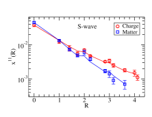
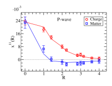
Figure 4: Ground state vector and scalar radial distributions and discretized exponential fits.

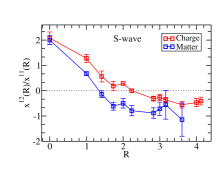
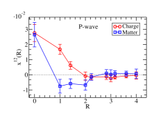
Figure 5: Radial distributions containing the first radially excited state (Ref. [2] for the S-wave).

The lattice measurements, i.e. the energy spectrum and the radial distributions, can be used to test potential models. There are several advantages for model makers: First of all, since the heavy quark is infinitely heavy, we have essentially a one-body problem. Secondly, on the lattice we know what we put in — one heavy quark and one light anti-quark — which makes the lattice system much more simple than the real world. We can, for example, try to use the Dirac equation to interpret the S- and P-wave distributions. Reasonable parameters can give a surprisingly good qualitative fit to the distributions measured on the lattice — see Fig. 6.

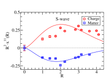
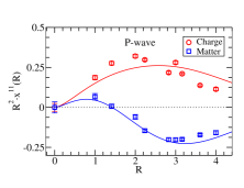
Figure 6: Dirac equation numerical solutions for a potential $V=-e/R+b\cdot R$ compared with lattice results. Here $e=0.6\cdot\hslash c$, $b=(500~{}\textrm{MeV})^{2}$ and $m=100$ MeV. $R$ is in lattice units ($a\approx 0.15$ fm).

3 Main conclusions

• There should be several narrow $B_{s}$ states, e.g. $0^{+}$ that lies below the $BK$ threshold.

• The spin-orbit splitting is very small.

• The radial distributions of S and P$-$ states can be qualitatively understood by using a Dirac equation model.

References

• [1] C. Michael and J. Peisa for UKQCD Collaboration, Phys. Rev. D 58, 34506 (1998).
• [2] A.M. Green, J. Koponen, C. Michael and P. Pennanen for UKQCD Collaboration, Phys. Rev. D 65, 014512 (2002) and Eur. Phys. J. C 28, 79 (2003), hep-lat/0206015
• [3] A.M. Green, J. Koponen, C. McNeile, C. Michael and G. Thompson for UKQCD Collaboration, Phys. Rev. D 69, 094505 (2004).
• [4] H. J. Schnitzer, Phys. Rev. D 18, 3482 (1978) and Phys. Lett. B 226, 171 (1989).