The two-grid algorithm confronts a shifted unitary orthogonal method

Abstract

In this paper I describe a new optimal Krylov subspace solver for shifted unitary matrices called the Shifted Unitary Orthogonal Method (SUOM). This algorithm is used as a benchmark against any improvement like the two-grid algorithm. I use the latter to show that the overlap operator can be inverted by successive inversions of the truncated overlap operator. This strategy results in large gains compared to SUOM.

It is well-known that overlap fermions [1] lead to much more expensive computations than standard fermions, i.e. Wilson or Kogut-Sussking fermions. This is obvious since for every application of the overlap operator an extra linear system solving is needed. For the time being, it seems that to get chiral symmetry at finite lattice spacing one should wait for a Petaflops computer being built.

However, algorithmic research is far from exhausted. In this paper I give an example that this is the case if one uses the two-grid algorithm [2]. Before I do this, I introduce briefly an optimal Krylov subspace solver for shifted unitary matrices.

1 SUOM: A NEW OPTIMAL KRYLOV SOLVER

Consider the task of solving the linear system:

$$Dx=b,~{}~{}~{}D=c_{1}\text{1\kern-2.41109ptl}+c_{2}V$$ (1.1)

where $V=\gamma_{5}$sign$(H_{W})$ is a unitary matrix, 1l the identity matrix, $H_{W}$ the Hermitian Wilson operator, $c_{1}=(1+m_{q})/2,c_{2}=(1-m_{q})/2$ and $m_{q}$ the bare fermion mass. The overlap operator $D$ is non-Hermitian. For such operators GMRES (Generalised Minimal Residual) and FOM (Full Orthogonalisation Method) are known to be the fastest. It is shown that when the norm-minimising process of GMRES is converging rapidly, the residual norms in the corresponding Galerkin process of FOM exhibit similar behaviour [3]. But they are based on long recurrences and thus require to store a large number of vectors of the size of matrix columns. However, exploiting the fact that the overlap operator is a shifted unitary matrix one can construct a GMRES type algorithm with short recurrences [4].

Similarly, a short recurrences algorithm can be obtained from FOM. The method is based on an observation of Rutishauser [5] that for upper Hessenberg unitary matrices one can write $H=LU^{-1}$, where $L$ and $U$ are lower and upper bidiagonal matrices. Applying this decomposition for the Arnoldi iteration:

$$VQ_{k}=Q_{k}H_{k}+h_{k+1,k}q_{k+1}e_{k}^{T}$$ (1.2)

one obtains an algorithm which constructs Arnoldi vectors $Q_{k}$ by short recurrences [6]:

$$VQ_{k}U_{k}=Q_{k}L_{k}+l_{k+1,k}q_{k+1}e_{k}^{T}.$$ (1.3)

Projecting the linear system (1.1) onto the Krylov subspace one gets:

$$(c_{1}\text{1\kern-2.41109ptl}_{k}+c_{2}L_{k}U_{k}^{-1})y_{k}=e_{1}$$ (1.4)

which can be equivalently written as:

$$(c_{1}U_{k}+c_{2}L_{k})z_{k}=e_{1},~{}~{}~{}y_{k}=U_{k}z_{k}.$$ (1.5)

Note that the matrix on the left hand side is tridiagonal. It can be shown that one can solve this system and therefore the original system using short recurrences [6]. The resulting algorithm is called the Shifted Unitary Orthogonal Method (SUOM) and is given below:

Algorithm 1    SUOM algorithm

  $\rho=||b||_{2};~{}q_{0}=b/\rho;~{}w_{0}=q_{0}$

  $l_{00}=q_{0}^{H}Vq_{0}$

  $\tilde{q}=Vq_{0}-l_{00}q_{0}$

  $l_{10}=||\tilde{q}||_{2};~{}q_{1}=\tilde{q}/l_{10}$

  $\tilde{l}_{00}=c_{1}+c_{2}l_{00}$

  $\alpha_{0}=\rho/\tilde{l}_{00};~{}x_{0}=\alpha_{0}w_{0};~{}r_{0}=b-\alpha_{0}Dw_{0}$

  for $~{}k=1,2,\ldots$ do

     $u_{k-1k}=-q_{k-1}^{H}Vq_{k}/q_{k-1}^{H}Vq_{k-1}$

     $l_{kk}=q_{k}^{H}Vq_{k}+u_{k-1k}q_{k}^{H}Vq_{k-1}$

     $\tilde{q}=(V-l_{kk})q_{k}+u_{k-1k}Vq_{k-1}$

     $l_{k+1k}=||\tilde{q}||_{2}$

     $q_{k+1}=\tilde{q}/l_{k+1k}$

     $\tilde{l}_{kk}=c_{1}+c_{2}l_{kk}-c_{1}c_{2}l_{kk-1}u_{k-1k}/\tilde{l}_{k-1k-1}$

     $\alpha_{k}=-c_{2}l_{kk-1}/\tilde{l}_{kk}\alpha_{k-1}$

     $w_{k}=q_{k}+u_{k-1k}q_{k-1}-c_{1}u_{k-1k}/\tilde{l}_{k-1k-1}w_{k-1}$

     $x_{k}=x_{k-1}+\alpha_{k}w_{k}$

     $r_{k}=r_{k-1}-\alpha_{k}Dw_{k}$

     Stop if $||r_{k}||_{2}<$ tol $\rho$

  end for

Note that in an actual implementation one can store $Vq_{k}$ and $Dw_{k}$ as separate vectors, which can be used in the subsequent iteration to compute $Dw_{k+1}$. Therefore only one multiplication by $V$ is needed at each step.

2 THE TWO-GRID ALGORITHM

A straightforward application of multigrid algorithms is hopeless in the presence of non-smooth gauge fields. However, the situation is different for the 5-dimensional formulation of chiral fermions where there are no gauge connections along the fifth dimension. Here, I will limit my discussion in the easiest case which consists of two grids: the “fine” grid, which is the continuum along the fifth coordinate and a coarse grid, which is the lattice discretisation of the “fine” grid.

I define chiral fermions on the coarse grid using truncated overlap fermions [7]. The corresponding 5-dimensional matrix ${\mathcal{M}}$ in blocked form is given by:

$$\small\begin{pmatrix}D_{W}-\text{1\kern-2.16997ptl}&(D_{W}+\text{1\kern-2.16997ptl})P_{+}&-m_{q}(D_{W}+\text{1\kern-2.16997ptl})P_{-}\\ (D_{W}+\text{1\kern-2.16997ptl})P_{-}&\ddots&\\ &\ddots&\ddots\\ -m_{q}(D_{W}+\text{1\kern-2.16997ptl})P_{+}&&D_{W}-\text{1\kern-2.16997ptl}\\ \end{pmatrix}$$

where $P_{\pm}=(\text{1\kern-2.41109ptl}_{4}+\gamma_{5})/2$. Let ${\mathcal{M}}_{1}$ be the above matrix but with bare quark mass $m_{q}=1$ and $P$ the permutation matrix:

$$\small\hskip 28.45274pt\begin{pmatrix}P_{+}&P_{-}&&\\ &P_{+}&\ddots&\\ &&\ddots&P_{-}\\ P_{-}&&&P_{+}\\ \end{pmatrix}$$

It can be shown that the following result hold [2, 8]:

Proposition 2.1

Let $P^{T}{\mathcal{M}}_{1}^{-1}{\mathcal{M}}P\chi=\eta$ be the linear system defined on the 5-dimensional lattice with $\chi=(y,\chi^{(2)},\ldots,\chi^{(N_{5})})^{T}$ and $\eta=(r,o,\ldots,o)^{T}$. Then $y$ is the solution of the linear system $D^{(N_{5})}y=r$, where $D^{(N_{5})}\rightarrow D$ as $N_{5}\rightarrow\infty$.

This result lends itself to a special two-grid algorithm [2, 8]. Indeed, $x_{5}=a_{5}$ is the (fifth Euclidean) coordinate of interest since it contains the information about the 4-dimensional physics.

Algorithm 2    The two-grid algorithm

  $x_{1}\in\mathbb{C}^{N};~{}r_{1}=b-Dx_{1};~{}\text{tol},\text{tol}_{0}\in\mathbb{R}_{+}$

  for $~{}i=1,2,\ldots$ do

     Let $\eta_{i}=(r_{i},o,\ldots,o)^{T}\in\mathbb{C}^{NN_{5}}$

     Let $\chi_{i+1}=(y_{i+1},\chi_{i+1}^{(2)},\ldots,\chi_{i+1}^{(N_{5})})^{T}\in\mathbb{C}^{NN_{5}}$

     Solve  ${\mathcal{M}}P\chi_{i+1}={\mathcal{M}}_{1}P\eta_{i}$ until

     $||{\mathcal{M}}_{1}P\eta_{i}-{\mathcal{M}}P\chi_{i+1}||_{2}<\text{tol}_{0}~{}||{\mathcal{M}}_{1}P\eta_{i}||_{2}$

     $x_{i+1}=x_{i}+y_{i+1}$

     $r_{i+1}=b-Dx_{i+1}$

     Stop if $||r_{i+1}||_{2}<$ tol $||b||_{2}$

  end for

One way of exploiting this is to use “decimation” over the fifth coordinate in order to get the 5d-vector $\eta$. Using proposition 2.1 one can evaluate directly the first 4d-component of $\eta$ by $r=b-Dx$, $x$ being an approximate solution. The rest can be padded with zero 4d-vectors. The second step is to solve the problem on the coarse grid. Finally, one can extract the 4d-solution $y$ on this grid and correct the “fine” grid solution by $x\leftarrow x+y$. In the second cycle one has to repeat the same decimation method, since the “fine” 5d-operator is not available. Hence, the whole scheme is a restarted two-grid algorithm, which is given here as Algorithm 2.

3 COMPARISON OF METHODS

In Fig. 1 is shown the convergence of variuos algorithms as a function of Wilson matrix-vector multiplication number on a fixed gauge background on a $8^{3}16$ lattice at $\beta=5.7$. The convergence is measured using the norm of the residual error. For the overlap matrix-vector multiplication is used the double pass Lanczos algorithm (without small eigenspace projection of $H_{W}$) as described in [9]. Together with the algorithms described in the previous sections Fig. 1 shows the performance of Conjugate Residuals (CR), Conjugate Gradients on Normal Equations (CGNE) and CG-CHI. The latter is the CGNE which solves simultaneously the decoupled chiral systems appearing in the matrix $D^{H}D$. One can observe a gain over CGNE which may be explained due to the reduced number of eigenvalues at each chiral sector. However, this gain is no more than $10\%$. On the other hand SUOM and CR preform rather similar with SUOM being slightly faster in this scale. The gain over CGNE is about a factor two. The Two-Grid algorithm performs the best with a gain of at least a factor 6 over SUOM and more than an order of magnitude over CGNE. This situation repeats itself for a different gauge configuration which is not shown here for the lack of space. However, if the projection of small eigenvalues is used the gain over SUOM/CR should be smaller since the Two-Grid algorithm is much less intensive in the application of the overlap operator. It is exactly the purpose of this comparison to make clear this feature of the Two-Grid algorithm. Finally, it is (not) surprising that SUOM and CR perform similarly: CR can be shown to be an efficient method for normal matrices. Since it is easier to implement CR is more appealing than other Krylov solvers.

The results of this work suggest that the full multigrid algorithm along the fifth dimension should be the next method to be explored.

Aknowledgements. The author would like to thank Andreas Kronfeld and LOC of Lattice 2004 for the kind support and Soros Foundation Albania for granting the travel to Fermilab.

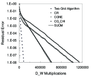
Figure 1: Norm of the residual as a function of the number of $D_{W}(M)$ multiplications for different algorithms for $M=-1.8$

References

- [1] H. Neuberger, Phys. Lett. B 417 (1998) 141
- [2] A. Boriçi, Phys. Rev. D62 (2000) 017505
- [3] J. Cullum and A. Greenbaum, SIAM J. Matrix Anal. Appl., V17, 2, pp. 223-247 (1996)
- [4] C. F. Jagels und L. Reichel, Num. Lin. Algeb. Appl., Vol. 1(6), 555-570 (1994) and G. Arnold et al, hep-lat/0311025
- [5] H. Rutishauser, Numer. Math. 9 (1966) 104
- [6] A. Boriçi, in preparation.
- [7] A. Boriçi, Nucl. Phys. Proc. Suppl. 83 (2000) 771-773
- [8] A. Boriçi, in V. Mitrjushkin and G. Schierholz (edts.), Lattice Fermions and Structure of the Vacuum, Kluwer Academic Publishers, 2000. See also A. Boriçi, hep-lat/0402035.
- [9] A. Boriçi, Phys. Lett. B453 (1999) 46-53