Study of the 2-d $CP(N-1)$ models at $\theta=0$ and $\pi$

Abstract

We present numerical results for 2-d $CP(N\!-\!1)$ models at $\theta\!=\!0$ and $\pi$ obtained in the D-theory formulation. In this formulation we construct an efficient cluster algorithm and we show numerical evidence for a first order transition for $CP(N\!-\!1\!\geq\!2)$ models at $\theta=\pi$. By a finite size scaling analysis, we also discuss the equivalence in the continuum limit of the D-theory formulation of the 2-d $CP(N-1)$ models and the usual lattice definition.

1 Introduction

$CP(N-1)$ models [1] are defined on the manifold $S^{2N-1}/S^{1}$ which is the coset space of the breaking of $SU(N)$ down to $U(N-1)$. The field $P(x)$ is parametrized by Hermitean $N\!\times\!N$ projector matrices, i.e. $P(x)^{2}=P(x)$ and $\mbox{Tr }P(x)=1$. The action is given by

$$S[P]=\frac{1}{g^{2}}\int\;dx\;\mbox{Tr}[\partial_{\mu}P(x)\partial_{\mu}P(x)],$$ (1)

and it is invariant under the global $\Omega\in SU(N)$ transformation $P(x)^{\prime}=\Omega P(x)\Omega^{+}$. The 2-d $CP(N-1)$ models are interesting toy-models of 4-d Yang-Mills theories. In fact, these two quantum field theories share several important features, including asymptotic freedom, the dynamical generation of a mass-gap and an instanton topological charge. In particular, this latter property leads to a non-trivial vacuum angle $\theta$ and allows to consider $CP(N-1)$ models in order to investigate $\theta$-vacuum effects. It has been conjectured that $CP(N-1)$ models have a phase transition at $\theta\!=\!\pi$. For $CP(1)\!=\!O(3)$ this phase transition is known to be second order with a vanishing mass-gap [2, 3, 4]. For $N\!>\!2$ the transition is conjectured to be first order [5, 6]. Studying these nonperturbative problems is highly nontrivial and one can eventually address these questions only numerically. However, the numerical simulation of $CP(N\!-\!1)$ models is not straightforward, even at $\theta=0$. In fact, in contrast to $O(N)$ models where the Wolff cluster algorithm [7] can be used, no efficient cluster algorithm is available [8, 9]. Still a rather efficient multi-grid algorithm was developed in [10]. At $\theta=\pi$ the numerical investigations become even more difficult due to a very severe sign problem. In fact, in this case, the topological sectors with even and odd charges have opposite Boltzmann weights and their contributions almost completely cancel in the partition function. This makes it exponentially hard to simulate the large lattices necessary to reach reliable conclusions on the phase structure. For this reason, efficient simulations at $\theta=\pi$ have been performed only in the $CP(1)=O(3)$ case by a Wolff-type meron-cluster algorithm [4]. Here we present results obtained with a method allowing to perform an unbiased and very accurate numerical study of any 2-d $CP(N-1)$ model at $\theta=0$ and $\pi$ [11]. Our method is based on the D-theory formulation of a field theory [12]. This is a different formulation than Wilson’s and consists in obtaining the continuous fields from the dimensional reduction of discrete variables. It provides an alternative lattice regularization of field theory but with the same continuum limit. More details on the results presented here can be found in [11].

2 $CP(N-1)$ models: D-theory formulation

In this section we discuss 2-d $CP(N\!-\!1)$ models in the D-theory formulation. The discrete variables we consider are $SU(N)$ quantum spins $T_{x}^{a}=\frac{1}{2}\lambda_{x}^{a}$, generators of the $SU(N)$ group $[T_{x}^{a},T_{y}^{b}]=i\delta_{xy}f_{abc}T_{x}^{c}$. The spins are located on the sites $x$ of a $L\times L^{\prime}$ periodic square lattice with $L\gg L^{\prime}$. Hence we have the geometry of a spin ladder consisting of $n=L^{\prime}/a$ transversely coupled spin chains of length $L$.

Figure 1: Spin ladder geometry: open circles form sublattice $A$, filled circles belong to sublattice $B$.

We consider n.n. couplings: antiferromagnetic along the chains and ferromagnetic between different chains. The lattice naturally decomposes into two sublattices $A$ and $B$. The spins in $A$ transform in the fundamental representation $\{N\}$, while those belonging to $B$ are in the conjugate one $\{\overline{N}\}$ and are described by $-T_{x}^{a*}$. The quantum spin ladder Hamiltonian is

$$H = -J\sum_{x\in A}[T_{x}^{a}T_{x+\hat{1}}^{a*}+T_{x}^{a}T_{x+\hat{2}}^{a}]$$ (2)

$$- J\sum_{x\in B}[T_{x}^{a*}T_{x+\hat{1}}^{a}+T_{x}^{a*}T_{x+\hat{2}}^{a*}],$$

where $J>0$, and $\hat{1}$ and $\hat{2}$ are unit-vectors in the $x$- and $y$-directions, respectively. The system has a global $SU(N)$ symmetry, i.e. $[H,T^{a}]=0$, with the total spin $T^{a}=\sum_{x\in A}T_{x}^{a}-\sum_{x\in B}T_{x}^{a*}$, satisfying the $SU(N)$ algebra $[T^{a},T^{b}]=if_{abc}T^{c}$. The quantum partition function at the temperature $T=1/\beta$ is then given by $Z=\mbox{Tr exp}(-\beta H)$.

Using the coherent state technique of [13] one finds that, at $T=0$ and for $L,L^{\prime}\rightarrow\infty$, the $SU(N)$ symmetry breaks down to $U(N-1)$. Thus there are massless Goldstone bosons described by fields $P\!\in\!SU(N)/U(N-1)=CP(N-1)$. When the $y$-direction is compactified to a finite extent $L^{\prime}$, the Coleman-Hohenberg-Mermin-Wagner theorem forbids massless excitations. Thus the Goldstone bosons pick up a nonperturbatively generated mass-gap $m=1/\xi$ and the correlation length $\xi$ is now finite. For sufficiently many transversely coupled chains, the correlation length becomes exponentially large, $\xi\gg L^{\prime}$, and the system both undergoes dimensional reduction and approaches the continuum limit. Using chiral perturbation theory, one finds that the lowest-order terms in the 2-d Euclidean effective action are given by

$$S[P]=\int dxdt\{\frac{1}{g^{2}}\;\mbox{Tr}[\partial_{\mu}P\partial_{\mu}P]-i\theta Q[P]\}.$$ (3)

where $Q[P]$ is the topological charge

$$Q[P]=\frac{1}{2\pi i}\int dxdt\;\epsilon_{\mu\nu}\mbox{Tr}[P\partial_{\mu}P\partial_{\nu}P],$$ (4)

and $\theta=n\pi$ is the vacuum angle. Hence, $\theta=0$ for even $n$ and $\theta=\pi$ for odd $n$.

3 The numerical study

One advantage of D-theory is that it is a formulation of a quantum field theory in terms of simple discrete degrees of freedom instead of the usual continuum classical fields. In particular, the partition function $Z$ of the $SU(N)$ quantum spin ladder can be written using a basis of discrete $SU(N)$ spin states: $q\in\{u,d,s,...\}$ on sublattice $A$ and $\overline{q}\in\{\overline{u},\overline{d},\overline{s},...\}$ on sublattice $B$. These can be simulated with the loop-cluster algorithm [14, 15]. The efficient cluster algorithm we have used in this study is a generalization to $SU(N)$ of the $SU(2)$ case [15].

The Hamiltonian (2) is the sum of 4 terms that we denote, respectively, with $H_{1},\ldots,H_{4}$: two of them ($H_{2}$, $H_{4}$) describe the ferromagnetic interaction while the other two ($H_{1}$, $H_{3}$) the antiferromagnetic one. Using the Trotter decomposition we write $Z$ as follows

$$Z=\lim_{M\rightarrow\infty}\mbox{Tr}\left[\mbox{e}^{-\epsilon H_{1}}\mbox{e}^{-\epsilon H_{2}}\mbox{e}^{-\epsilon H_{3}}\mbox{e}^{-\epsilon H_{4}}\right]^{M}$$ (5)

where we have introduced $4M$ slices in the $\beta$-direction with spacing $\epsilon=\beta J/M$. Inserting complete sets of states between the exponential factors, one obtains that the only non-vanishing transfer matrix elements are given by

$$\langle q^{i},q^{i}|\mbox{e}^{-\epsilon H_{2}}|q^{i},q^{i}\rangle=\mbox{e}^{\epsilon\frac{N-1}{2N}}$$ (6)

$$\langle q^{i},q^{j\neq i}|\mbox{e}^{-\epsilon H_{2}}|q^{i},q^{j\neq i}\rangle=(\mbox{e}^{\epsilon\frac{N-1}{2N}}+\mbox{e}^{-\epsilon\frac{N+1}{2N}})/2$$

$$\langle q^{i},q^{j\neq i}|\mbox{e}^{-\epsilon H_{2}}|q^{j\neq i},q^{i}\rangle=(\mbox{e}^{\epsilon\frac{N-1}{2N}}-\mbox{e}^{-\epsilon\frac{N+1}{2N}})/2$$

$$\langle q^{i},\overline{q}^{i}|\mbox{e}^{-\epsilon H_{1}}|q^{i},\overline{q}^{i}\rangle=(\mbox{e}^{\frac{\epsilon N}{2}}+N-1)\,\mbox{e}^{-\frac{\epsilon}{2N}}/N$$

$$\langle q^{i},\overline{q}^{j\neq i}|\mbox{e}^{-\epsilon H_{1}}|q^{i},\overline{q}^{j\neq i}\rangle=\mbox{e}^{-\frac{\epsilon}{2N}}$$

$$\langle q^{i},\overline{q}^{j\neq i}|\mbox{e}^{-\epsilon H_{1}}|q^{j\neq i},\overline{q}^{i}\rangle=(\mbox{e}^{\frac{\epsilon N}{2}}-1)\,\mbox{e}^{-\frac{\epsilon}{2N}}/N$$

The transfer matrix elements for $H_{3}$ and $H_{4}$ can be obtained by substituting $H_{1}\!\rightarrow\!H_{3}$, $H_{2}\!\rightarrow\!H_{4}$ and $q\!\leftrightarrow\!\overline{q}$. With these matrix elements at hand, the construction of the quantum spin cluster and its updating proceeds like in the $SU(2)$ case. One can also avoid the slicing in the $\beta$-direction operating directly in continuous Euclidean time [16].

We have used this cluster algorithm to investigate if $CP(N-1)$ models with $N>2$ have a first order phase transition at $\theta=\pi$ where the charge conjugation symmetry $C$ is spontaneously broken. An order parameter for such a phase transition would be the topological charge $Q[P]$ which indeed is $C$-odd: $Q[^{C}P]=Q[P^{*}]=-Q[P]$. However $Q$ is defined only in the framework of the target continuum theory. In the discrete spin system we define as order parameter $Q[q,\overline{q}]$ the number of spin flips in a configuration. $Q[q,\overline{q}]$ gets a contribution +1 if a pair of n.n. spins along the $x$-direction, $q_{x}\overline{q}_{x+\hat{1}}$, flips to another state, $q_{x}^{\prime}\overline{q}_{x+\hat{1}}^{\prime}$, at some moment in time. A spin flip from $\overline{q}_{x}q_{x+\hat{1}}$ to $\overline{q}_{x}^{\prime}q_{x+\hat{1}}^{\prime}$ instead contributes $-1$. In the quantum spin ladder, charge conjugation corresponds to replacing each spin state $q_{x}$ by $q_{x+\hat{1}}$ and, indeed, $Q[q,\overline{q}]$ changes sign under this operation while the action remains invariant.

We have simulated $SU(N)$ quantum spin ladders for $N=3,4$, and 5, with $n=L^{\prime}/a\in\{2,3,...,7\}$. Our simulations confirm the existence of a first order phase transition with spontaneous $C$-breaking at $\theta=\pi$ for all $N>2$. As expected, there is no phase transition at $\theta=0$. Figure 2 shows Monte Carlo time histories of $Q[q,\overline{q}]$ for $SU(4)$ spin ladders with $n=3$ and 4. For $n=3$ one observes two coexisting phases with spontaneous $C$-breaking, while for $n=4$ there is only one $C$-symmetric phase. Similar results have been obtained in the other cases studied.

Finally, we have verified explicitly that the $CP(N-1)$ models in Wilson’s and in the D-theory formulation have the same continuum limit. In order to do this we have compared a physical quantity – namely the universal finite-size scaling function $F(\xi(L)/L)=\xi(2L)/\xi(L)$ – measured in both frameworks. In [11] we show the excellent agreement between the results obtained in these two formulations.

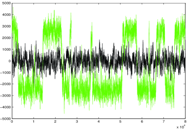
Figure 2: Monte Carlo time histories of $Q[q,\overline{q}]$ for the $CP(3)$ model at $\theta=0$ and $\pi$.

References

- [1] A. D’Adda, P. Di Vecchia, and M. Lüscher, Nucl. Phys. B146 (1978) 63; Nucl. Phys. B152 (1979) 125.
- [2] F. D. M. Haldane, Phys. Rev. Lett. 50 (1983) 1153.
- [3] I. Affleck and E. Lieb, Lett. Math. Phys. 12 (1986) 57.
- [4] W. Bietenholz, A. Pochinsky, and U.-J. Wiese, Phys. Rev. Lett. 75 (1995) 4524.
- [5] I. Affleck, Nucl. Phys. B305 [FS23] (1988) 582; Phys. Rev. Lett. 66 (1991) 2429.
- [6] N. Seiberg, Phys. Rev. Lett. 53 (1984) 637.
- [7] U. Wolff, Phys. Rev. Lett. 62 (1989) 361.
- [8] K. Jansen and U.-J. Wiese, Nucl. Phys. B370 (1992) 762.
- [9] S.Caracciolo et al, Nucl.Phys. B403(1993)475.
- [10] M. Hasenbusch and S. Meyer, Phys.Rev.Lett. 68 (1992) 435; Phys. Rev. D45 (1992) 4376.
- [11] B. B. Beard et al., arXiv:hep-lat/0406040.
-
[12]
S. Chandrasekharan and U.-J. Wiese, Nucl. Phys. B492 (1997) 455;
R. Brower, S. Chandrasekharan, and U.-J. Wiese, Phys. Rev. D60 (1999) 094502;
R. Brower et al., Nucl. Phys. B693 (2004) 149. - [13] N. Read and S. Sachdev, Nucl. Phys. B316 (1989) 609.
-
[14]
H. G. Evertz, G. Lana, and M. Marcu, Phys. Rev. Lett. 70 (1993) 875;
H. G. Evertz, Adv. Phys. 52 (2003) 1. - [15] U.-J. Wiese and H.-P. Ying, Z. Phys. B93 (1994) 147.
- [16] B. B. Beard and U.-J. Wiese, Phys. Rev. Lett. 77 (1996) 5130.