Improving Algorithms to Compute All Elements of the Lattice Quark Propagator

Abstract

We present a new exact algorithm for estimating all elements of the quark propagator. The advantage of the method is that the exact all-to-all propagator is reproduced in a large but finite number of inversions. The efficacy of the algorithm is tested in Monte Carlo simulations of Wilson quarks in quenched QCD. Applications that are difficult to probe with point propagators are discussed.

1 INTRODUCTION

The discovery of exactly chirally symmetric fermions on the lattice has triggered intensive research in the development of algorithms to simulate dynamical Ginsparg-Wilson fermions on the lattice. In light of recent work in this area, we anticipate that there will be a limited number of expensive, full QCD configurations in the near future. One would like to extract all the information that one can from these lattices without being restricted by point propagators, which would appear highly wasteful considering the cost to generate the configurations. Point propagators do not require massive computing power but restrict the physics one has access to, mainly the flavour non-singlet spectrum. They also restrict the interpolating operator basis used to produce early plateaux in effective masses, for instance, since a new inversion must be performed for every operator that is not restricted to a single lattice point. Variational methods would be much more powerful with the use of all-to-all propagators.

All-to-all propagators [1, 2, 3, 4, 5, 6] provide a solution to these problems, but are usually too expensive to compute exactly as this requires an unrealistic number of quark inversions. Stochastic estimates tend to be very noisy and variance reduction techniques are crucial in order to separate the signal from the noise. In this paper we propose an exact algorithm to compute the all-to-all propagator utilizing the idea of low-mode dominance corrected by a stochastic estimator which yields the exact all-to-all propagator in a finite number of quark inversions.

2 THEORY AND NOTATION

2.1 Spectral Decomposition

Theoretical arguments, backed up by numerical evidence [7, 8], indicate that the low lying eigenmodes of the Hermitian Dirac operator captures much of the important infrared physics in hadronic interactions. It would be desirable to take advantage of this fact and solve exactly for as many of the eigenmodes as possible to estimate the all-to-all quark propagator.

To this end, we define the Hermitian Dirac operator $Q=\gamma_{5}M$ where $M$ is the usual Dirac operator. The truncated representation of the quark propagator is then given by,

$$\bar{Q}_{0}=\sum_{i}^{N_{ev}}\frac{1}{\lambda_{i}}v^{(i)}(\vec{y},y_{0})\otimes v^{(i)}(\vec{x},x_{0})^{\dagger}\,,$$ (1)

where $Qv^{(i)}=\lambda_{i}v^{(i)}$. The truncation at an arbitrary number, $N_{ev}$, of eigenvectors, however, leaves the theory non-unitary, making it mandatory to correct it.

2.2 Dilution (Noisy Estimators)

The standard method of estimating the all-to-all quark propagator is to sample the vector space stochastically. One generates an ensemble of random noise vectors, $\{\eta_{[1]},\cdots,\eta_{[N_{r}]}\}$, with the property

$$\langle\!\langle\eta(x)\!\otimes\!\eta(y)^{\dagger}\rangle\!\rangle\propto\delta_{x,y}\,,$$ (2)

where $\langle\!\langle\cdots\rangle\!\rangle$ denotes average over noise samples. The solution for each vector is obtained in the usual way,

$$\psi_{[r]}(x)=Q^{-1}\eta_{[r]}(y)\,.$$ (3)

The all-to-all quark propagator is estimated as

$$\begin{split}Q^{-1}&=\langle\!\langle\psi\!\otimes\!\eta^{\dagger}\rangle\!\rangle\\ &\simeq\frac{1}{N_{r}}\sum_{r}^{N_{r}}\psi_{[r]}(y)\otimes\eta_{[r]}(x)^{\dagger}\,.\end{split}$$ (4)

This method is noisy because it relies on delicate cancellations in the ${\mathcal{O}}(1)$ noise over many samples to find the signal, which falls off exponentially with the separation. We propose to remove the ${\mathcal{O}}(1)$ random noise by “diluting” the noise vector according to some dilution scheme resulting in an exponential gain in the variance. A particularly important example of dilution for measuring temporal correlations in hadronic quantities is “time dilution” where the noise vector is broken up into pieces which only have support on a single timeslice each,

$$\eta(\vec{x},t)=\sum_{j=0}^{Nt-1}\eta^{(j)}(\vec{x},t)\,,$$ (5)

where $\eta^{(j)}(\vec{x},t)=0$ unless $t=j$.

Each diluted source is inverted resulting in $N_{t}$ pairs of vectors, $\{\psi^{(i)}(\vec{x},t),\eta^{(i)}(\vec{x},t)\}$, which then gives an unbiased estimator of $\langle\psi\bar{\psi}\rangle$ with a single noise source,

$$Q^{-1}=\sum_{i=0}^{N_{t}-1}\psi^{(i)}(\vec{x},t)\otimes\eta^{(i)}(\vec{x}_{0},t_{0})^{\dagger}\,.$$ (6)

We show the effect of time dilution on a pseudoscalar propagator on a $12^{3}\times 24$ lattice in Fig. 1. The triangles are the average of 24 noise sources without any dilution and the circles are from a single noise source which has been time-diluted. This particular scenario is analogous to the “wall source on every timeslice” method used by the authors of Ref. [1] to estimate the disconnected diagrams appearing in hadronic scattering length calculations. Our method is, however, more general and can be extended to the spin, color and space components of the source vector. The “homeopathic” limit of this dilution procedure results in the exact all-to-all propagator in a finite number of steps (Fig. 2). This limit cannot be reached in practice on realistic lattices, but the path of dilution may be optimized so that the noise from the gauge fields dominate the errors in the hadronic quantities of interest with only a small, managable number of fermion matrix inversions.

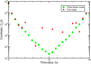
Figure 1: The psuedoscalar propagator computed with and without time dilution.

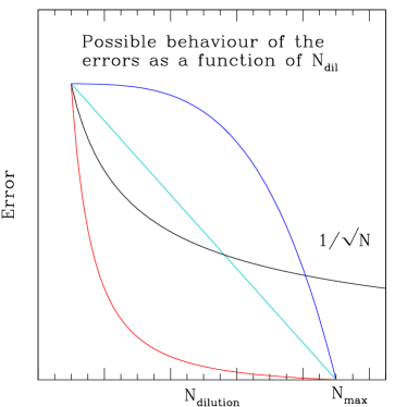
Figure 2: A cartoon of possible deviations of the stochastic estimates of the exact solution (at $N_{d}=N_{\text{max}}$) for different dilution paths. Simply adding noise vectors will give a $1/\sqrt{N}$ behaviour.

2.3 ‘Hybrid’ Method

The evidence that much of the hadronic physics we would like to extract from the lattice is in the low-lying eigenmodes of the (Hermitian) Dirac operator suggests that one try to calculate as many as possible of the low modes exactly and correct for the truncation with the noisy method. This gives rise to two concerns: firstly, the correction should leave the exactly solved low-lying modes intact; and secondly, it should not introduce large uncertanties in the process. We propose that the stochastic method with noise dilution is a natural way to accomodate both of those concerns.

First, we note that the exact $N_{ev}$ low eigenmodes obtained separately naturally divide $Q$ into two subspaces, $Q=Q_{0}+Q_{1}$, defined by

$$Q_{0} =\sum_{i=1}^{N_{ev}}\lambda_{i}v^{(i)}\otimes v^{(i)\dagger}\,,$$ (7)

$$Q_{1} =\sum_{j=N_{ev}+1}^{N}\lambda_{j}v^{(j)}\otimes v^{(j)\dagger}\,.$$ (8)

Similarly, the quark propagator is broken up into two pieces, $Q^{-1}=\bar{Q}_{0}+\bar{Q}_{1}$, where $\bar{Q}_{0}$ is given by Eq. (1) and $\bar{Q}_{1}$ is the remaining unknown piece. We correct for the truncation and estimate $\bar{Q}_{1}$ using the stochastic method, $\bar{Q}_{1}=\langle\!\langle\psi\!\otimes\!\eta^{\dagger}\rangle\!\rangle$ with $N_{r}$ noise vectors, $\{\eta_{[1]},\cdots,\eta_{[N_{r}]}\}$. The solutions are given by

$$\psi_{[r]}=\left(Q^{-1}{\mathcal{P}}_{1}\right)\eta_{[r]}=Q^{-1}\left({\mathcal{P}}_{1}\eta_{[r]}\right)\,,$$ (9)

where ${\mathcal{P}}_{1}$ is the projection operator

$${\mathcal{P}}_{1}={\bf 1}-{\mathcal{P}}_{0}={\bf 1}-\sum_{j=1}^{N_{ev}}v^{(j)}\otimes v^{(j)\dagger}\,.$$ (10)

Note that Eq. (9) follows from the identity $Q^{-1}{\mathcal{P}}_{1}=\bar{Q}_{1}$. As was mentioned earlier, the idea of dilution will be applied to the stochastic estimation of $\bar{Q}_{1}$. Each random noise vector, $\eta_{[r]}$, that is generated will be diluted and orthogonalized (wrt ${v^{(i)}}$) so that it can be used to obtain $\psi_{[r]}$. In other words, we now have the following set of noise vectors:

$$\left\{\left(\eta_{[1]}^{(1)},\cdots,\eta_{[N_{r}]}^{(1)}\right),\cdots,\left(\eta_{[1]}^{(N_{d})},\cdots,\eta_{[N_{r}]}^{(N_{d})}\right)\right\}\,,$$

where the upper indices denote the dilution and the lower indices label the different noise samples. We note that the noise vectors are mutually orthogonal to each other due to the dilution before an average over different random vectors are taken, i.e.,

$$\eta_{[r]}^{(i)}(\vec{x},t)\otimes\eta_{[s]}^{(j)}(\vec{y},t^{\prime})^{\dagger}\propto\delta^{ij}.$$ (11)

This results in smaller variance than the standard method which mixes noise, as Eq. (2) shows.

There is a natural way to combine the two methods to estimate the all-to-all quark propagator. The similarity in the structure of Eq. (1) and Eq. (4) suggests that one construct the following “hybrid list” for the source and solution vectors:

$$w^{(i)} =\biggl{\{}\frac{v^{(1)}}{\lambda_{1}},\cdots,\frac{v^{(N_{ev})}}{\lambda_{N_{ev}}},\eta^{(1)},\cdots,\eta^{(N_{d})}\biggr{\}}$$ (12)

$$u^{(i)} =\biggl{\{}v^{(1)},\cdots,v^{(N_{ev})},\psi^{(1)},\cdots,\psi^{(N_{d})}\biggr{\}}$$ (13)

where the indices run over $N_{HL}=N_{ev}+N_{d}$ elements. The master formula for the unbiased, variance reduced estimate of the all-to-all quark propagator is then given by

$$M^{-1}=\sum_{i=1}^{N_{HL}}u^{(i)}(\vec{x},x_{4})\otimes w^{(i)}(\vec{y},y_{4})^{\dagger}\gamma_{5}\,.$$ (14)

Using the pion as an example, we can demonstrate how unitarity is recovered from the truncated propagator. In Fig. 3, we show the effective mass from the truncated propagator and from the hybrid method with a time, spin, color and space (even-odd) diluted noise vector. The truncated propagator, which approaches the asymptotic value from below, is corrected by the addition of the diluted noisy propagator.

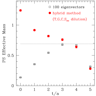
Figure 3: The effective mass from 100 eigenvectors and from the hybrid method with 100 eigenvectors and a time-diluted noise vector. The lattice size is $6^{3}\times 12$.

3 QCD IMPLEMENTATION

All-to-all propagators not only expand the range of applications accessible in lattice QCD but also considerably simplify the construction of hadronic interpolating operators. A pseudoscalar correlator is constructed in the following way with traditional, point-to-all quark propagators,

$$C=M^{-1}(\vec{x},t;\vec{0},0)^{\dagger\ ij}_{\ \alpha\beta}\;M^{-1}(\vec{x},t;\vec{0},0)^{ji}_{\beta\alpha}\,.$$ (15)

The construction of a better operator is awkward at best since the operator at timeslice $t$ is constructed from various components of the quark propagator connecting the source and sink. All-to-all propagators eliminate this complication as the operator at timeslice $t$ is constructed from vectors on that timeslice,

$$\begin{split}{\mathcal{O}}_{PS}^{(i,j)}(\vec{x},t)&=(w^{(i)}_{[r_{1}]}(\vec{x},t)^{\dagger}\gamma_{5})\gamma_{5}u^{(j)}_{[r_{2}]}(\vec{x},t)\\ &=w^{(i)}_{[r_{1}]}(\vec{x},t)^{\dagger}u^{(j)}_{[r_{2}]}(\vec{x},t)\,,\end{split}$$ (16)

where the extra factor of $\gamma_{5}$ comes from the use of the Hermitian Dirac matrix, $\gamma_{5}M$. For complicated operators such as those used to project out hybrid/exotic states, this is a much needed simplification. For example, an interpolating operator for the exotic hybrid $1^{-+}$ can be constructed from combinations of gluonic paths projecting out the relevant quantum numbers [9]. One term in such a sum may be

$$w^{[i]}(\vec{x})^{\dagger}U_{z}(\vec{x})U_{y}(\vec{x}+\hat{z})U_{z}^{\dagger}(\vec{x}+\hat{e}_{y})u^{[j]}(\vec{x}+\hat{e}_{y})\,,$$ (17)

where all the variables are located on a single timeslice. A standard P-wave state may for example be constructed as follows,

$${\mathcal{O}}_{P}^{(i,j)}(\vec{x},t)=w^{(i)}(\vec{x},t)^{\dagger}(D_{k}u^{(j)})(\vec{x},t)\,,$$ (18)

where $D_{k}$ is the covariant derivative.

Using all-to-all propagators, correlation functions are also constructed in an intuitive manner. Hadronic correlation functions are obtained by correlating interpolating operators sitting at different timeslices, e.g.

$$C(t,t_{0})=\sum_{i,j}^{N_{HL}}{\mathcal{O}}_{[r_{1},r_{2}]}^{(i,j)}(t){\mathcal{O}}_{[r_{2},r_{1}]}^{(j,i)}(t_{0})\,$$ (19)

for isovector two-point correlators (propagators).

Noting that this is simply a contraction of the source and solution vectors with an outer sum over the hybrid list indices, this gives even greater scope for simplification. Once the machinery of the hybrid list summation is set up in the program, it becomes a black box to the end user who simply supplies the subroutines to create the required operators from the quark, antiquark and gluon fields on a timeslice.

For isoscalar mesons, the disconnected part of the propagator must be included, yielding the following contraction,

$$\left\{w^{(i)}_{[2]}(t)^{\dagger}\gamma_{5}\Gamma u^{(j)}_{[1]}(t)\right\}\left\{w_{[1]}^{(j)}(t_{0})^{\dagger}\gamma_{5}\Gamma^{\dagger}u_{[2]}^{(i)}(t_{0})\right\}\\ -\left\{w_{[1]}^{(j)}(t)^{\dagger}\gamma_{5}\Gamma u_{[1]}^{(j)}(t)\right\}\left\{w_{[2]}^{(i)}(t_{0})^{\dagger}\gamma_{5}\Gamma^{\dagger}u_{[2]}^{(i)}(t_{0})\right\}\,.$$ (20)

4 TESTS

We use the Wilson action to illustrate the effectiveness of the variance reduction although it is expected to work even better for a chiral action and light quarks. The simulation parameters are shown in Table 1.

Table 1: Fermion run parameters. The values for $m_{\pi},m_{\rho}$ are taken from Ref. [11].

$n_{x}^{3}\times n_{t}$	$\kappa$	$am_{\pi}$	$am_{\rho}$	$m_{\pi}/m_{\rho}$
$6^{3}\times 12$	0.1600	0.69	0.80	0.86
$12^{3}\times 24$	0.1600	0.69	0.80	0.86
$12^{3}\times 24$	0.1663	0.38	0.62	0.61
$12^{3}\times 24$	0.1675	0.30	0.60	0.50

In order to demonstrate the efficacy of the noise dilution method, we perform an “equal cost” comparison test. Equal cost here shall mean the same number of inversions performed, disregarding the sparseness of the source vector. For example, an even-odd dilution in space results in twice as many inversions as the one without, hence two independent sets of time diluted noise vectors are generated to compare the noise in the effective mass of the psuedoscalar. As we have seen that no signal is obtained otherwise, all noise vectors have been time diluted. The results are shown in Fig. 4. The noise diluted errors consistently show smaller errors than the standard stochastic method.

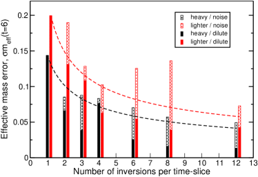
Figure 4: Equal cost test of the pion effective mass at timeslice 6.

At this point, one may note that the isovector correlation function (when both quarks are saved as all-to-all) involves a large number ($N_{HL}\times N_{HL}$) of contractions. We can take advantage of having saved different random source/solution samples by reusing them in the contraction. In other words, one can generate $N_{R}$ samples of noise vectors, $\eta_{[r]}$, and save the corresponding solutions, $\psi_{[r]}$ to disk and perform the contraction,

$$C=\sum_{r,s}w^{\dagger}_{[r]}u_{[s]}(t)w^{\dagger}_{[s]}u_{[r]}(t_{0})\,,$$ (21)

yielding $\sim\!N_{R}^{2}$ samples of the pion correlation function. The errors correspondingly decrease faster than the naïve $1/\sqrt{N_{R}}$, although the measurements are correlated. We have seen in our preliminary tests that the gain in error reduction is comparable to some dilution choices. It is clear that if one can afford to save the noise/solution vectors onto disk, then this is a straightforward method of variance reduction.

We have performed some spectroscopy calculations using the idea of dilution. Standard meson spectroscopy including pions, rhos, heavy exotic hybrids (with two different operators) and standard P-wave states were studied. For the P-wave states in particular, it is difficult to get a good overlap using point propagators. The effective masses for all the particles are shown in Fig. 5 and Fig. 6. Although in this test study we only used 10 quenched gauge configurations, we have a surprisingly good signal for P-waves as well as the extremely heavy hybrid states. Furthermore, decay constants can be extracted from point–smeared and smeared–smeared correlators if all-to-all propagators are used [10].

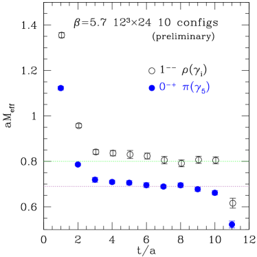
Figure 5: The pion and rho meson effective masses from 10 configurations on a $\beta=5.7$, $12^{3}\times 24$ lattice.

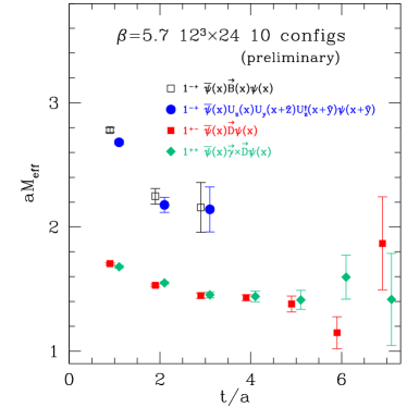
Figure 6: Preliminary results for a variety of P-wave states. The staple hybrid operators actually use a length-2 staple.

5 SUMMARY

We have presented a new algorithm to estimate the all-to-all propagator. All-to-all propagators make it possible to make use of all the available information in a gauge configuration, which considering the cost to generate full QCD configurations may be of crucial importance. They are also a necessary ingredient in flavour singlet physics.

All-to-all propagators have a further advantage over point propagators in that operator construction is considerably simplified: The operators are constructed in a natural way from local fields, and extended operators used in variational methods may be employed at no additional cost.

We have presented evidence that diluting stochastic estimators in time, colour, spin or other variables gives less variance than traditional noisy estimators. This is not unexpected, since dilution will yield the exact all-to-all propagator in a finite number of iterations. More work is needed to determine the optimal dilution path for different observables.

The hybrid method allows one to extract the important physics from low-lying eigenmodes and combine this with a noisy correction in a natural way. This may be implemented in such a way that the user can be blind to the details of the dilution and eigenvector list.

Preliminary tests of the algorithm have been presented with small lattices and a small number of configurations. We find that the algorithm works as expected for standard light-light, static-light and exotic meson spectroscopy. Further work will include higher statstics on lighter masses as well as tests on disconnected diagrams.

References

- [1] Y. Kuramashi et al., Phys. Rev. Lett. 71 (1993) 2387.
- [2] S. J. Dong and K. F. Liu, Phys. Lett. B 328 (1994) 130, hep-lat/9308015.
- [3] G. M. de Divitiis et al., Phys. Lett. B 382 (1996) 393, hep-lat/9603020.
- [4] C. Michael and J. Peisa, Phys. Rev. D 58 (1998) 034506, hep-lat/9802015.
- [5] A. Duncan and E. Eichten, Phys. Rev. D 65 (2002) 114502, hep-lat/0112028.
- [6] M.J. Peardon, Nucl. Phys. Proc. Suppl. 106 (2002) 3, hep-lat/0201003.
- [7] A. Duncan et al., Phys. Rev. D 59 (1999) 014505, hep-lat/9806020.
- [8] H. Neff et al., Phys. Rev. D 64 (2001) 114509, hep-lat/0106016.
- [9] P. Lacock et al., Phys. Rev. D 54 (1996) 6997, hep-lat/9605025.
- [10] TrinLat, S.M. Ryan et al., these proceedings.
- [11] F. Butler et al., Nucl. Phys. B430 (1994) 179, hep-lat/9405003.