DESY 04-176, SFB/CPP-04-48, HU-EP-04/52 hep-lat/0409058
September 2004
Signal at subleading order in lattice HQET

Abstract

We discuss the correlators in lattice HQET that are needed to go beyond the static theory. Based on our implementation in the Schrödinger functional we focus on their signal-to-noise ratios and check that a reasonable statistical precision can be reached in quantities like $f_{\mathrm{B}_{\mathrm{s}}}$ and $M_{\mathrm{B^{\star}}}\!-\!M_{\mathrm{B}}$.

1 INTRODUCTION

The physics of mixings and decays of B-mesons is crucial for a determination of several entries of the CKM-matrix, e.g. $V_{ub}$. To relate experimental observations to Standard Model parameters, transition elements of the effective weak Hamiltonian must be computed in a reliable fully non-perturbative framework, e.g. on the lattice.

Since the large mass of the $b$-quark evades a direct treatment at lattice spacings $a^{-1}\!=\!2-4\,\,\mathrm{GeV}$, effective field theory methods are invoked. The one tried first is the static approximation which is the leading order of an expansion in the inverse heavy mass, i.e. the leading order of HQET [1]. Here, the heavy flavor field $\psi_{\mathrm{h}}$ satisfies $(1+\gamma_{0})\psi_{\mathrm{h}}=2\psi_{\mathrm{h}}$ and has a discretized action

$$S_{\mathrm{h}}^{\mathrm{EH}}\!\! \!\!=\!\! \!\!a^{4}\sum_{x}\bar{\psi}_{\mathrm{h}}(x)D_{0}\psi_{\mathrm{h}}(x)$$ (1)

$$D_{0}\psi_{\mathrm{h}}(x)\!\! \!\!=\!\! \!\![\psi_{\mathrm{h}}(x)\!-\!U^{\dagger}(x\!-\!a\hat{\mathbf{0}},0)\psi_{\mathrm{h}}(x\!-\!a\hat{\mathbf{0}})]/a\;.$$

A non-perturbative renormalization of the effective theory – including the subleading terms – is possible, i.e. divergences can be subtracted implicitly through a direct matching against QCD in a small volume, and very precise results at short ($x_{0}\!<\!0.5\,\mathrm{fm}$) distances may be obtained [2]. One of the advantages of such a strategy is that the theory maintains a well-defined continuum limit, while this would not be true, if the matching was performed to any fixed order in perturbation theory. We consider this important.

There are, however, some intrinsic difficulties with this approach. The first one is the statistical noise in correlators at large ($x_{0}\!>\!0.5\,\mathrm{fm}$) euclidean distances. Brute force is no solution, since the noise-over-signal ratio grows exponentially in $x_{0}$. This is related to the $1/a$ divergence that has been subtracted. If the HQET approach is extended beyond the leading order, $1/a^{n}$ divergences are implicitly canceled, and the obvious fear is that the noise problem will be even worse. The second difficulty relates to the fact that any limited precision in the matching will translate into additional uncertainties of all quantities in the large volume; hence devising good matching conditions is an important task. Here, we shall address point one, i.e. the statistical precision that can be reached in typical correlators at the next-to-leading order in the HQET expansion.

2 CORRELATION FUNCTIONS

The Schrödinger functional (SF) master formula for the heavy meson decay constant

$${F_{\mathrm{B}}\sqrt{m_{\mathrm{B}}}\over 2L^{3/2}}\!=\!\left\{\begin{array}[]{l}\!\!\!-Z_{\mathrm{A}}{f_{\mathrm{A}}(T/2)\over\sqrt{f_{1}}}\\ \!\!\!-C_{\mathrm{PS}}(M_{\mathrm{b}}/\Lambda)Z_{\mathrm{A}}^{\mathrm{stat}}{f_{\mathrm{A}}^{\mathrm{stat}}(T/2)\over\sqrt{f_{1}^{\mathrm{stat}}}}+\mathrm{O}({1\over m})\!\!\!\!\!\end{array}\right.$$

relates the expression in the relativistic formulation to that in the HQET approach. In the latter, the correlation functions at leading order are

$$f_{\mathrm{A}}^{\mathrm{stat}}(x_{0})\! \!=\! \!-{1\over 2}\langle A_{0}^{\mathrm{stat}}(x)O\rangle$$ (2)

$$f_{1}^{\mathrm{stat}}\! \!=\! \!-{1\over 2}\langle O^{\prime}O\rangle$$ (3)

with the static-light axial current

$$A_{0}^{\mathrm{stat}}(x)=\bar{\psi}(x)\gamma_{0}\gamma_{5}\psi_{\mathrm{h}}(x)$$ (4)

and the boundary operators

$$O\! \!=\! \!\sum_{\mathbf{y},\mathbf{z}}\bar{\zeta}_{\mathrm{h}}(\mathbf{y})\gamma_{5}\omega(\mathbf{y}\!-\!\mathbf{z})\zeta(\mathbf{z})$$

$$O^{\prime}\! \!=\! \!\sum_{\mathbf{y}^{\prime},\mathbf{z}^{\prime}}\bar{\zeta}^{\prime}(\mathbf{y}^{\prime})\gamma_{5}\omega(\mathbf{y}^{\prime}\!-\!\mathbf{z}^{\prime})\zeta^{\prime}_{\mathrm{h}}(\mathbf{z}^{\prime})$$

on the bottom and top ($x_{0}\!=\!0,T$) of the SF-box.

The idea of lattice HQET at subleading order is to expand the Lagrangian (we include coefficients for subsequent renormalization)

$$L_{\mathrm{HQET}}=L_{\mathrm{stat}}-{\tilde{\omega}^{\mathrm{kin}}\over 2m}\bar{\psi}_{\mathrm{h}}\mathbf{D}^{2}\psi_{\mathrm{h}}-{\tilde{\omega}^{\mathrm{spin}}\over 2m}\bar{\psi}_{\mathrm{h}}\mathbf{\sigma\!\cdot\!B}\psi_{\mathrm{h}}$$

in the exponent and to treat the new terms as insertions in any correlator. Expanding consistently means that one keeps just terms in $1/m$, no products $\mathrm{O}(1/m^{2})$. The correlator $f_{\mathrm{A}}^{\mathrm{stat}}$ is thus augmented by $\tilde{\omega}^{\mathrm{kin/spin}}/(2m)$ times

$$f_{\mathrm{A}}^{\mathrm{kin/spin}}(x_{0})\!=\!-{1\over 2}\langle A_{0}^{\mathrm{stat}}(x)\sum_{u}X^{\mathrm{kin/spin}}(u)O\rangle$$ (5)

with $X^{\mathrm{kin}}(u)\!=\!\bar{\psi}_{\mathrm{h}}(u)\mathbf{D}^{2}\psi_{\mathrm{h}}(u)$ as bulk insertion or $X^{\mathrm{spin}}(u)\!=\!\bar{\psi}_{\mathrm{h}}(u)\mathbf{\sigma\!\cdot\!B}\psi_{\mathrm{h}}(u)$, and ditto for $f_{1}^{\mathrm{stat}}$. The dimension 5 pieces of the Lagrangian appear only as insertions, and this is crucial for the renormalizability [to order $1/m$] of the theory.

The expansion of $f_{\mathrm{A}}$ to order $1/m$ reads

$$f_{\mathrm{A}}\!\propto\!f_{\mathrm{A}}^{\mathrm{stat}}\Big{\{}1\!+\!{\alpha^{(1)}\over\alpha^{(0)}}\!{\delta\!f_{\mathrm{A}}^{\mathrm{stat}}\over f_{\mathrm{A}}^{\mathrm{stat}}}\!+\!\omega^{\mathrm{kin}}{f_{\mathrm{A}}^{\mathrm{kin}}\over f_{\mathrm{A}}^{\mathrm{stat}}}\!+\!\omega^{\mathrm{spin}}{f_{\mathrm{A}}^{\mathrm{spin}}\over f_{\mathrm{A}}^{\mathrm{stat}}}\Big{\}}\!$$

where $\omega^{\mathrm{kin}}\!=\!\tilde{\omega}^{\mathrm{kin}}/(2m)$ ($=\!{1\over 2}\omega_{2}^{(1)}$ in the notation of [2]) and similarly for $\omega^{\mathrm{spin}}$. An analogous expression (without the $\delta\!f_{\mathrm{A}}^{\mathrm{stat}}$ piece defined in [3]) replaces $f_{1}^{\mathrm{stat}}$. The coefficients $\alpha^{(0/1)},\omega^{\mathrm{kin/spin}}$ are functions of $M_{b}a,g_{0}^{2}$ and may be determined as in [2]. Hence

$${F_{\mathrm{B}}\sqrt{m_{\mathrm{B}}}\over 2L^{3/2}}\! \!=\! \!-{\alpha^{(0)}\!f_{\mathrm{A}}^{\mathrm{stat}}\over\sqrt{f_{1}^{\mathrm{stat}}}}\Big{\{}1+{\alpha^{(1)}\over\alpha^{(0)}}{\delta\!f_{\mathrm{A}}^{\mathrm{stat}}\over f_{\mathrm{A}}^{\mathrm{stat}}}+$$

$$\!\omega^{\mathrm{kin}}R^{\mathrm{kin}}(T/2)+\omega^{\mathrm{spin}}R^{\mathrm{spin}}(T/2)\Big{\}}$$

where

$$R^{\mathrm{kin}}={f_{\mathrm{A}}^{\mathrm{kin}}\over f_{\mathrm{A}}^{\mathrm{stat}}}\!-\!{1\over 2}{f_{1}^{\mathrm{kin}}\over f_{1}^{\mathrm{stat}}}\,,\;R^{\mathrm{spin}}={f_{\mathrm{A}}^{\mathrm{spin}}\over f_{\mathrm{A}}^{\mathrm{stat}}}\!-\!{1\over 2}{f_{1}^{\mathrm{spin}}\over f_{1}^{\mathrm{stat}}}\;.$$

In the same way, an effective mass $m_{\mathrm{eff}}(x_{0})\!=\!a^{-1}\log(f_{\mathrm{A}}(x_{0})/f_{\mathrm{A}}(x_{0}\!+\!a))$ is $1/m$-expanded as

$$m_{\mathrm{eff}}(x_{0})\! \!=\! \!m_{\mathrm{eff}}^{\mathrm{stat}}(x_{0})+\delta m+$$ (7)

$$\!\omega^{\mathrm{kin}}r^{\mathrm{kin}}(x_{0})+\omega^{\mathrm{spin}}r^{\mathrm{spin}}(x_{0})$$

with $m_{\mathrm{eff}}^{\mathrm{stat}}(x_{0})$ from $f_{\mathrm{A}}^{\mathrm{stat}}(x_{0})$ and

$$r^{\mathrm{kin}}(x_{0})\! \!=\! \!a^{-1}\Big{[}{f_{\mathrm{A}}^{\mathrm{kin}}(x_{0})\over f_{\mathrm{A}}^{\mathrm{stat}}(x_{0})}-{f_{\mathrm{A}}^{\mathrm{kin}}(x_{0}\!+\!a)\over f_{\mathrm{A}}^{\mathrm{stat}}(x_{0}\!+\!a)}\Big{]}$$

$$r^{\mathrm{spin}}(x_{0})\! \!=\! \!a^{-1}\Big{[}{f_{\mathrm{A}}^{\mathrm{spin}}(x_{0})\over f_{\mathrm{A}}^{\mathrm{stat}}(x_{0})}-{f_{\mathrm{A}}^{\mathrm{spin}}(x_{0}\!+\!a)\over f_{\mathrm{A}}^{\mathrm{stat}}(x_{0}\!+\!a)}\Big{]}\;.$$

Here, the contribution ${\alpha^{(1)}\over\alpha^{(0)}}[{\delta\!f_{\mathrm{A}}^{\mathrm{stat}}(x_{0})\over f_{\mathrm{A}}^{\mathrm{stat}}(x_{0})}-{\delta\!f_{\mathrm{A}}^{\mathrm{stat}}(x_{0}\!+\!a)\over f_{\mathrm{A}}^{\mathrm{stat}}(x_{0}\!+\!a)}]$ has been suppressed, since in the plateau region the two terms would cancel, while $r^{\mathrm{kin/spin}}$ approach a constant value each.

3 NUMERICAL RESULTS

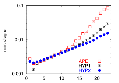
Figure 1: Noise-over-signal ratio for the heavy-light correlator $f_{\mathrm{A}}^{\mathrm{kin}}$, using three discretizations of the heavy propagator. Similar graphs are obtained at leading order in the $1/m$ expansion [3].

The problem of large fluctuations in the static-light propagator was solved by modifying the covariant derivative in (1). As shown in [3], an APE- or HYP-smeared link $V^{\dagger}(x\!-\!a\hat{\mathbf{0}},0)$ instead of $U^{\dagger}$ leads to an improvement in the noise-over-signal ratio of $f_{\mathrm{A}}^{\mathrm{stat}}(x_{0})$ which grows exponentially with $x_{0}$ while the discretization errors remain at the same level. Fig. 1 shows that a similar improvement is found at subleading order in the $1/m$ expansion. HYP-links [4] with $(\alpha_{1},\alpha_{2},\alpha_{3})\!=\!(1.0,1.0,0.5)$ do better than those with $(\alpha_{1},\alpha_{2},\alpha_{3})\!=\!(0.75,0.6,0.3)$, which, in turn, are better than APE-links [5] with staple-only contribution and no $SU(3)$-projection. The same ordering was found at leading order.

At this point we cannot compute the subleading contribution to $f_{\mathrm{B_{s}}}$, since the matching coefficients $\alpha^{(0/1)},\omega^{\mathrm{kin/spin}}$ have not yet been determined, but we can assess the statistical error of such a contribution. Our figure and numbers stem from a quenched simulation in a $16^{3}\!\times\!24$ SF-box at $\beta\!=\!6.0$ with $\kappa\!\simeq\!\kappa_{\mathrm{strange}}$ and 5600 measurements, and we shall quote only the results for the improved HYP-parametrization. For the two correction terms in (2) we find the values $aR^{\mathrm{kin}}\!=\!-0.78(14)$, $aR^{\mathrm{spin}}\!=\!-0.83(03)$.

For an interpretation of their statistical errors, we need a rough figure for the coefficients $\omega^{\mathrm{kin/spin}}$. Up to typical (logarithmically $a$-dependent) renormalization factors of order one, they can be estimated by their tree-level values $a^{-1}\omega^{\mathrm{kin/spin}}\!\simeq\!1/(2am)\!\simeq\!0.2$ (from $a^{-1}\!\simeq\!2\,\mathrm{GeV}$ and $m\!\simeq\!5\,\mathrm{GeV}$). In addition, the renormalization of $R^{\mathrm{kin/spin}}$ does require power divergent subtractions, but they are contained in $\alpha^{(0)}$ (for which, therefore, a tree-level estimate would be no good).

From $\omega^{\mathrm{kin/spin}}\!\simeq\!0.2$ one gets a statistical error of the kinetic contribution of 3% and an error of the spin contribution of 0.6% in expression (2). Neglecting uncertainties in the $\alpha^{(0/1)}$ and $\omega^{\mathrm{kin/spin}}$, it appears that already with the methods applied here, one can compute $f_{\mathrm{B_{s}}}$ at subleading order in the HQET expansion in such a way that the noise in the dimension 5 correlators increases the error by $\sim$3-4 percentage points.

A simpler application, where even a first estimate may be given, is the vector-pseudoscalar splitting $M_{\mathrm{B^{\star}}}\!-\!M_{\mathrm{B}}$. This effect sets in at subleading order in the HQET expansion,

$$M_{\mathrm{B^{\star}}}-M_{\mathrm{B}}\!=\!{4\over 3}\omega^{\mathrm{spin}}r^{\mathrm{spin}}(x_{0})$$ (8)

and has first been estimated in a lattice computation in [6]. Our result for the large-$x_{0}$ asymptotic is $a^{2}r^{\mathrm{spin}}\!=\!0.060(5)$. With $a^{-1}\omega^{\mathrm{spin}}\!\simeq\!0.2$ one gets $M_{\mathrm{B^{\star}}}\!-\!M_{\mathrm{B}}\!=\!0.016(1)(2\!\,\mathrm{GeV})\!=\!0.032(3)\,\mathrm{GeV}$, which should be compared to the experimental result $0.046\,\mathrm{GeV}$. Hence, the lattice value falls short by about a third. Whether this reflects a large renormalization factor (similar to $c_{\mathrm{SW}}$), a slow convergence of the HQET expansion or a genuine quenching artefact remains to be seen, although the results of [7] render the second explanation rather unlikely. We emphasize that these figures are just indicative; reliable numbers can be given only when $\omega^{\mathrm{spin}}$ has been determined and smaller lattice spacings have been considered.

4 CONCLUSION

We have attempted a first test with correlator ratios needed to compute observables in the heavy-light system beyond the static approximation. The natural fear that they will, for large euclidean distances, be even noisier than the leading order piece seems not to become true. This is because the reduction of the noise-over-signal ratio via a better HQ-discretization works more efficiently at subleading order. The statistical precision may be further improved, e.g. by employing a smaller time extent in $f_{1}^{\mathrm{stat}}$ and $f_{1}^{\mathrm{kin/spin}}$ (together with a careful choice of the wave function, see [3]) or by the methods of [8]. We conclude that lattice HQET at subleading order looks promising enough to motivate further studies.

We thank A. Shindler and M. Della Morte for checks on the implementation and discussions.

References

• [1] E. Eichten and B. Hill, Phys. Lett. B 234, 511 (1990).
• [2] J. Heitger and R. Sommer, JHEP 0402, 022 (2004) [hep-lat/0310035].
• [3] M. Della Morte, S. Dürr, J. Heitger, H. Molke, J. Rolf, A. Shindler and R. Sommer, Phys. Lett. B 581, 93 (2004) [hep-lat/0307021].
• [4] A. Hasenfratz and F. Knechtli, Phys. Rev. D 64, 034504 (2001) [hep-lat/0103029].
• [5] [APE Collab.] M. Albanese et al., Phys. Lett. B 192, 163 (1987).
• [6] M. Bochicchio et al., Nucl. Phys. B 372, 403 (1992).
• [7] J. Heitger, A. Jüttner, R. Sommer and J. Wennekers, hep-ph/0407227.
• [8] A.M. Green et al., Phys. Rev. D 69, 094505 (2004) [hep-lat/0312007].