Remarks on the discretization of physical momenta in lattice QCD

Abstract

The calculation on the lattice of cross–sections, form–factors and decay rates associated to phenomenologically relevant physical processes is complicated by the spatial momenta quantization rule arising from the introduction of limited box sizes in numerical simulations. A method to overcome this problem, based on the adoption of two distinct boundary conditions for two fermions species on a finite lattice, is here discussed and numerical results supporting the physical significance of this procedure are shown.

1 The problem

In the formulation of quantum field theories on a lattice the introduction of a finite volume is unavoidable when numerical simulations are used as tool of investigation. As a consequence of the limited box size, spatial momenta come out to be quantized accordingly to the choice of the boundary conditions.

The momentum quantization represents a severe limitation in various phenomenological applications by making impossible, in the great majority of the cases, to calculate cross–sections, decay–rates and form–factors in the interesting kinematical region or at the physical values of the masses of the particles involved in the processes. In this talk it is discussed a method, previously introduced in ref. [1], that allows to overcome these difficulties. The idea consists in using the dependence of the momentum quantization condition upon the choice of the boundary conditions (BC) and in requiring different fermion species to satisfy different BC.

2 The way out

In order to clarify the dependence of the momentum quantization rule upon the choice of the boundary conditions let us first consider the case of a particle satisfying periodic boundary conditions (PBC). For a fermionic field $\psi(x)$ on a 4–dimensional finite volume of topology $T\times L^{3}$ with PBC in the spatial directions one has

$$\psi(x+\vec{e}_{i}\ L)=\psi(x)\;,\qquad i=1,2,3$$ (1)

This condition can be re-expressed by Fourier transforming both members of the previous equation

$$\int{d^{4}p\ e^{-ip(x+\vec{e}_{i}\ L)}\ \tilde{\psi}(p)}=\int{d^{4}p\ e^{-ipx}\ \tilde{\psi}(p)}$$ (2)

and implies

$$e^{ip_{i}L}=1\quad\Longrightarrow\quad p_{i}=\frac{2\pi\ n_{i}}{L}$$ (3)

where the $n_{i}$’s are integer numbers. The authors of [2, 3, 4, 5, 6, 7, 8, 9] have considered a generalized set of boundary conditions, that here we call $\theta$–boundary conditions ($\theta$–BC), depending upon the choice of a topological 3–vector $\vec{\theta}$

$$\psi(x+\vec{e}_{i}\ L)=e^{i\theta_{i}}\ \psi(x)\;,\qquad i=1,2,3$$ (4)

The modification of the boundary conditions affects the zero of the momentum quantization rule. Indeed, by re-expressing equation (4) in Fourier space, as already done in the case of PBC in equation (2), one has

$$e^{i(p_{i}-\frac{\theta_{i}}{L})L}=1\quad\Longrightarrow\quad p_{i}=\frac{\theta_{i}}{L}+\frac{2\pi\ n_{i}}{L}$$ (5)

It comes out that the spatial momenta are still quantized as for PBC but shifted by an arbitrary continuous amount ($\theta_{i}/L$). The physical significance of this continuous shift in the allowed momenta becomes manifest, from the theoretical point of view, by realizing that eq. (4) is the condition satisfied by the electron wavefunctions in a periodic solid crystal accordingly to the well known Bloch’s theorem. Indeed, quarks on a lattice experience a periodic potential (the gauge fields) exactly as the electrons do in a crystal and the results of the Bloch’s theorem apply straight forwardly also to the lattice fields.

The generalized $\theta$–dependent boundary conditions of equation (4) can be implemented by making a unitary Abelian transformation on the fields satisfying $\theta$–BC

$$\psi(x)\quad\longrightarrow\quad{\mathcal{U}}\ (\theta,x)\psi(x)=e^{-\frac{i\theta x}{L}}\ \psi(x)$$ (6)

As a consequence of this transformation the resulting field satisfies periodic boundary conditions but obeys a modified Dirac equation

$$S[\bar{\psi},\psi] \rightarrow$$ (7)

$$\rightarrow \sum_{x,y}{\bar{\psi}(x)\ {\mathcal{U}}(\theta,x)D(x,y){\mathcal{U}}^{-1}(\theta,y)\ \psi(y)}$$

$$= \sum_{x,y}{\bar{\psi}(x)\ D_{\theta}(x,y)\ \psi(y)}$$

where the $\theta$–dependent lattice Dirac operator $D_{\theta}(x,y)$ is obtained by starting from the preferred discretization of the Dirac operator and by modifying the definition of the covariant lattice derivatives (see ref. [1] for details).

3 Numerical tests

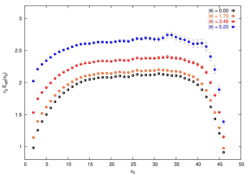
Figure 1: Effective energies $E_{eff}^{ij}(\theta,a;x_{0})$ at fixed cut–off. The results correspond to the simulation done at $\beta=6.211$ with $r_{0}\ m_{1}^{RGI}=0.655$ and $r_{0}\ m_{2}^{RGI}=0.354$. Similar figures could have been shown for other combinations of the simulated quark masses and for the other values of the bare coupling.

In order to prove numerically that the term $\vec{\theta}/L$ acts as a true physical momentum, one can study the energy of a meson made up by two different quarks with different $\theta$–BC for the two flavors. In the following we work in the $O(a)$–improved Wilson–Dirac lattice formulation of the QCD within the Schrödinger Functional formalism but, we want to stress that the use of $\theta$–BC in the spatial directions is completely decoupled from the choice of time boundary conditions and can be profitably used outside the Schrödinger Functional formalism, for example in the case of standard periodic time boundary conditions. Let us consider the following correlators

$$f_{P}^{ij}(\theta;x_{0})=$$

$$=-\frac{a^{6}}{2}\sum_{\vec{y},\vec{z},\vec{x}}{\langle\ \bar{\zeta}_{i}(\vec{y})\gamma_{5}\zeta_{j}(\vec{z})\ \bar{\psi}_{j}(x)\gamma_{5}\psi_{i}(x)\ \rangle}$$ (8)

where $i$ and $j$ are flavor indices, all the fields satisfy periodic boundary conditions and the two flavors obey different $\theta$–modified Dirac equations, as explained in eq. (7). In practice it is adequate to choose the flavor $i$ with $\theta=0$, i.e. with ordinary PBC, and the flavor $j$ with $\theta\neq 0$. After the Wick contractions the pseudoscalar correlator of equation (8) reads

$$f_{P}^{ij}(\theta;x_{0})=$$

$$=\frac{a^{6}}{2}\sum_{\vec{y},\vec{z},\vec{x}}\mbox{Tr}\;{\langle\gamma_{5}S_{j}(\theta;\vec{z},x)\gamma_{5}S_{i}(0;x,\vec{y})\rangle}$$ (9)

where $S(\theta;x,y)$ and $S(0;x,y)$ are the inverse of the $\theta$–modified and of the standard Wilson–Dirac operators respectively. Note that the projection on the momentum $\vec{\theta}/L$ of one of the quark legs in equation (9) it is not realized by summing on the lattice points with an exponential factor but it is encoded in the $\theta$–dependence of the modified Wilson–Dirac operator and, consequently, of its inverse $S(\theta;x,y)$. This correlation is expected to decay exponentially at large times as

$$f_{P}^{ij}(\theta;x_{0})\qquad\stackrel{{\scriptstyle x_{0}\gg 1}}{{\longrightarrow}}\qquad f_{ij}\ e^{-ax_{0}E_{ij}(\theta,a)}$$ (10)

where, a part from corrections proportional to the square of the lattice spacing, $E_{ij}$ is the physical energy of the mesonic state. After the continuum extrapolations one has to recover the expected relativistic dispersion relations

$$E_{ij}^{2}=M_{ij}^{2}+\left(\frac{\vec{\theta}}{L}\right)^{2}$$ (11)

where $M_{ij}$ is the mass of the pseudoscalar meson made of a $i$ and a $j$ quark anti–quark pair.

All the numerical results are obtained in the quenched approximation of the QCD. We have done simulations on a physical volume of topology $T\times L^{3}$ with $T=2L$ and linear extension $L=3.2\ r_{0}$, where $r_{0}$ is defined in [10]. All the missing parameters of the simulations are given in table 1 of ref. [1].

Setting the lattice scale by using the physical value $r_{0}=0.5$ fm, the expected values of the physical momenta associated with our choices of $\vec{\theta}$ are calculated according to the following relation

$$|\vec{p}|=\frac{|\vec{\theta}|}{L}\simeq 0.125\ |\vec{\theta}|\;\mbox{GeV}=\left\{\begin{array}[]{l}0.000\\ 0.217\\ 0.433\\ 0.650\\ \end{array}\right.\;\mbox{GeV}$$ (12)

where $L\simeq 1.6$ fm. These values have to be compared with the value of the lowest physical momentum allowed on this finite volume in the case of periodic boundary conditions, i.e. $|\vec{p}|\simeq 0.785$ GeV.

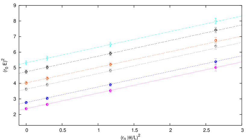
Figure 2: Continuum dispersion relations. The data correspond to different combinations of the simulated quark masses and reproduce very well the expected theoretical behavior, i.e. straight lines having as intercepts the meson masses and as angular coefficients one (see eq. 11).

At fixed cut–off, for each combination of flavor indices and for each value of $\vec{\theta}$ we have extracted the effective energy from the correlations of eq. (8), $f_{P}^{ij}(\theta;x_{0})$. In fig. 1 we show this quantity for the simulation performed at $\beta=6.211$ corresponding to $r_{0}\ m_{1}^{RGI}=0.655$ and $r_{0}\ m_{2}^{RGI}=0.354$, for each simulated value of $\vec{\theta}$. As can be seen the correlations with higher values of $|\vec{\theta}|$ are always greater than the corresponding ones with lower values of the physical momentum, a feature that will be confirmed in the continuum limit. Being interested in the ground state contribution to the correlation of eq. (8), we have averaged the effective energies over a ground state plateau of physical length depending upon the quark flavors and we have extrapolated the resulting quantities, $E^{ij}(\theta,a)$, to the continuum (see ref. [1] for details).

The continuum results verify very well the dispersion relations of equation (11) as can be clearly seen from fig. 2 in which the square of $E^{ij}(\theta)$ for various combinations of the flavor indices is plotted versus the square of the physical momenta $|\vec{\theta}|/L$. The plotted lines have not been fitted but have been obtained by using as intercepts the simulated meson masses and by fixing their angular coefficients to one.

References

- [1] G. M. de Divitiis, R. Petronzio and N. Tantalo, Phys. Lett. B595 (2004) 408, hep-lat/0405002.
- [2] K. Jansen et al., Phys. Lett. B372 (1996) 275, hep-lat/9512009.
- [3] A. Bucarelli et al., Nucl. Phys. B552 (1999) 379, hep-lat/9808005.
- [4] Zeuthen-Rome / ZeRo, M. Guagnelli et al., Nucl. Phys. B664 (2003) 276, hep-lat/0303012.
- [5] P.F. Bedaque, (2004), nucl-th/0402051.
- [6] D.J. Gross and Y. Kitazawa, Nucl. Phys. B206 (1982) 440.
- [7] J. Kiskis, R. Narayanan and H. Neuberger, Phys. Rev. D66 (2002) 025019, hep-lat/0203005.
- [8] J. Kiskis, R. Narayanan and H. Neuberger, Phys. Lett. B574 (2003) 65, hep-lat/0308033.
- [9] A. Roberge and N. Weiss, Nucl. Phys. B275 (1986) 734.
- [10] R. Sommer, Nucl. Phys. B411 (1994) 839, hep-lat/9310022.