Numerical test of Polyakov loop models in high temperature SU(2)

Abstract

We study the compatibility of effective mean-field models of the Polyakov loop for the deconfined phase of SU(N) pure gauge theories with lattice data obtained for the case of SU(2), in the temperature range $T_{c}\div 4.8T_{c}$.

1 INTRODUCTION

It has been suggested in several papers (see Ref. [1]) that the deconfined phase of SU(N) pure gauge theories could be described by an effective mean-field theory of the Polyakov loop, possessing global Z(N) invariance. Through this effective theory, a relation can be established between the pressure of the gluon gas and the Polyakov loop. If the phase transition is second order as for SU(2) or “weakly” first order as for SU(3), this effective theory can be written near the transition in terms of the first few powers of the Polyakov loop and of its complex conjugate. In this case, the relation between pressure and Polyakov loop becomes very simple and its compatibility with lattice data can be easily tested.

In this study, we have considered the case of SU(2) pure gauge theory on a 16${}^{3}\times 4$ lattice with the standard Wilson action, in the temperature range $T_{c}\div 4.80\,T_{c}$. Although lattice effects are large for the Wilson action with $N_{\tau}=4$ sites in the time direction, the shape of the behavior of pressure and Polyakov loop with the temperature should not be different from the cases of larger values of $N_{\tau}$, as seen in SU(3) [2].

2 LATTICE DETERMINATIONS

The pressure of the gluon gas is given by

$$\frac{p}{T^{4}}=-\left.\frac{f}{T^{4}}\right|_{\beta_{0}}^{\beta}=N_{\tau}^{4}\int_{\beta_{0}}^{\beta}d\beta^{\prime}[\langle S_{0}\rangle-\langle S_{T}\rangle]\;,$$ (1)

where $S_{0}$ ($S_{T}$) is the action density at zero (non-zero) temperature, $\beta_{0}$ is an arbitrarily chosen value, small enough that the integrand function at this point has become zero. Monte Carlo simulations were performed on $16^{4}$ lattices for zero-temperature (typical statistics 30K), and on $16^{3}\times 4$ lattices for non-zero temperature (typical statistics 80K). Numerical results for $N_{\tau}^{4}[\langle S_{0}\rangle-\langle S_{T}\rangle]$ were interpolated by cubic splines before the numerical integration which led to the pressure (Fig. 1). As an estimate of the uncertainty for the pressure, we calculated also the integral by interpolating the data for $N_{\tau}^{4}[\langle S_{0}\rangle-\langle S_{T}\rangle]$ with the broken line connecting the 1$\sigma$ upper (lower) bound of each determination. The correspondence between $\beta$ and the temperature has been established using the interpolating ansatz of Ref. [3], which makes use of the known [4] critical couplings on lattices with $N_{\tau}$=4, 5, 6, 8, 16.

We considered both the charge-1 and charge-2 Polyakov loops, given respectively by $l_{1}=\frac{1}{2}\langle\mbox{Tr}L(\vec{x})\rangle$ and $l_{2}=\frac{1}{2}\langle\mbox{Tr}L(\vec{x})^{2}\rangle-\left[\frac{1}{2}\langle\mbox{Tr}L(\vec{x})\rangle\right]^{2}$, with $L(\vec{x})=\prod_{n_{4}=1}^{N_{\tau}}U_{4}(\vec{x},n_{4})$. We observe that $l_{2}$ is Z(2)-invariant and is connected to the Polyakov loop in the adjoint color representation by $l_{\mbox{\footnotesize adj}}=1+4l_{2}/3$. In Fig. 2 we show the behavior of $l_{1}^{4}$, $l_{1}^{6}$ and $l_{2}$ with $\beta$. We observe that $l_{1}^{4}$ goes linear in the region $2.30\,\raisebox{-2.58334pt}{${\textstyle\stackrel{{\scriptstyle<}}{{\sim}}}$}\,\beta\,\raisebox{-2.58334pt}{${\textstyle\stackrel{{\scriptstyle<}}{{\sim}}}$}\,2.37$ (corresponding to $T_{c}\,\raisebox{-2.58334pt}{${\textstyle\stackrel{{\scriptstyle<}}{{\sim}}}$}\,T\,\raisebox{-2.58334pt}{${\textstyle\stackrel{{\scriptstyle<}}{{\sim}}}$}\,1.27\,T_{c}$) and in the region $2.45\,\raisebox{-2.58334pt}{${\textstyle\stackrel{{\scriptstyle<}}{{\sim}}}$}\,\beta\,\raisebox{-2.58334pt}{${\textstyle\stackrel{{\scriptstyle<}}{{\sim}}}$}\,2.80$ (corresponding to $1.65\,T_{c}\,\raisebox{-2.58334pt}{${\textstyle\stackrel{{\scriptstyle<}}{{\sim}}}$}\,T\,\raisebox{-2.58334pt}{${\textstyle\stackrel{{\scriptstyle<}}{{\sim}}}$}\,4.80\,T_{c}$). Moreover, $l_{2}$ goes to $-3/4$ in the confined phase, thus implying $l_{\mbox{\footnotesize adj}}\to 0$ in that phase (for details on the behavior of $l_{\mbox{\footnotesize adj}}$ across the transition, see Ref. [5]).

Figure 1: The three solid curves represent $p/T^{4}$ and its uncertainty; the vertical lines represent the critical couplings on lattices with $N_{\tau}$=4, 5, 6, 8, 16 [4].

Figure 2: $l_{1}^{4}$, $l_{1}^{6}$ and $l_{2}$ vs $\beta$ on a $16^{3}\times 4$ lattice.

3 POLYAKOV LOOP MODELS IN PURE GAUGE SU(2)

Mean-field theory, dimensional analysis, Z(2) symmetry, reality of $l_{1}$ in SU(2), power expansion in $l_{1}^{2}$ imply the following simple form for the effective free energy:

$${\cal V}=\left(-\frac{b_{2}}{2}\,l_{1}^{2}+\frac{b_{4}}{4}\,l_{1}^{4}\right)\,T^{4}\;,\;\;\;b_{2}>0\;,\;b_{4}>0\;.$$ (2)

The applicability domain of this model (called model A in the following) should be a region above $T_{c}$, but not so close to $T_{c}$ that mean-field is spoiled, in which $l_{1}$ is small enough to make $l_{1}^{6}$, $l_{1}^{8}$, … terms negligible. The minimum of ${\cal V}$ is obtained for $l_{1}^{2}=b_{2}/b_{4}$ and leads to

$$\frac{p}{T^{4}}=-\frac{{\cal V}_{\mbox{\footnotesize min}}}{T^{4}}=\frac{b_{4}}{4}\,l_{1}^{4}\;.$$ (3)

According to this model, for constant $b_{4}$, $p/T^{4}$ should go linear with $l_{1}^{4}$. We find that the function $(b_{4}/4)\,l_{1}^{4}$ fits the lattice data for the pressure in the region $2.33\leq\beta\leq 2.37$, i.e. $1.11\,T_{c}\,\raisebox{-2.58334pt}{${\textstyle\stackrel{{\scriptstyle<}}{{\sim}}}$}\,T\,\raisebox{-2.58334pt}{${\textstyle\stackrel{{\scriptstyle<}}{{\sim}}}$}\,1.27\,T_{c}$, with $b_{4}=261.1(6.7)$ and $\chi^{2}$/(d.o.f.)=0.79 (see Fig. 3).

For high temperatures, one could expand the effective free energy in powers of $(1-l_{1}^{2})$, thus getting

$${\cal V}_{\mbox{\footnotesize HT}}=\left(C-\frac{b_{2}}{2}\,l_{1}^{2}+\frac{b_{4}}{4}\,l_{1}^{4}\right)\,T^{4}\;,$$ (4)

which leads to

$$\frac{p}{T^{4}}=-\frac{{\cal V}_{\mbox{\footnotesize HT,min}}}{T^{4}}=C+\frac{b_{4}}{4}\,l_{1}^{4}\;.$$ (5)

There is compatibility of this functional form with lattice data for constant values of $C$ and $b_{4}$ in the region $2.60\leq\beta\leq 2.80$, i.e. $2.63\,T_{c}\,\raisebox{-2.58334pt}{${\textstyle\stackrel{{\scriptstyle<}}{{\sim}}}$}\,T\,\raisebox{-2.58334pt}{${\textstyle\stackrel{{\scriptstyle<}}{{\sim}}}$}\,4.80\,T_{c}$, with $b_{4}=19.7(4.8)$, $C=0.547(31)$ and $\chi^{2}$/(d.o.f.)=0.18 (see Fig. 3).

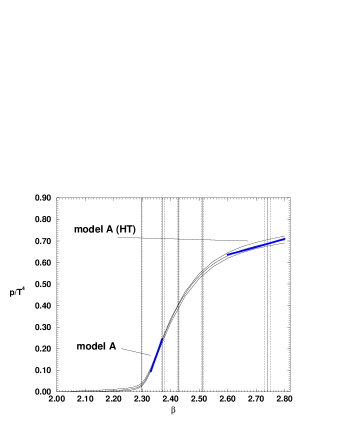
Figure 3: Comparison of the model A, for both low and high temperature regimes, with lattice data for the pressure.

As a first variant of the model A, we consider the inclusion of the $l_{1}^{6}$ term in the effective free energy (model B):

$${\cal V}=\left(-\frac{b_{2}}{2}\,l_{1}^{2}+\frac{b_{4}}{4}\,l_{1}^{4}+\frac{b_{6}}{6}\,l_{1}^{6}\right)\,T^{4}\;,$$ (6)

which leads to

$$\frac{p}{T^{4}}=-\frac{{\cal V}_{\mbox{\footnotesize min}}}{T^{4}}=\frac{b_{6}}{3}\,l_{1}^{6}+\frac{b_{4}}{4}\,l_{1}^{4}\;.$$ (7)

We find compatibility with the lattice data for the pressure over a wider region than in the case of model A, more precisely in the range $2.32\leq\beta\leq 2.70$, i.e. $1.07\,T_{c}\,\raisebox{-2.58334pt}{${\textstyle\stackrel{{\scriptstyle<}}{{\sim}}}$}\,T\,\raisebox{-2.58334pt}{${\textstyle\stackrel{{\scriptstyle<}}{{\sim}}}$}\,3.56\,T_{c}$, with $b_{4}=350.3(6.1)$, $b_{6}=-1158(33)$ and $\chi^{2}$/(d.o.f.)=0.73. A negative value for $b_{6}$ would be problematic if the absolute value of $l_{1}$ would be allowed to become arbitrarily large, which is not the case here. For high temperatures, using $(1-l_{1}^{2})$ as expansion parameter we get

$$\frac{p}{T^{4}}=-\frac{{\cal V}_{\mbox{\footnotesize HT,min}}}{T^{4}}=C+\frac{b_{6}}{3}\,l_{1}^{6}+\frac{b_{4}}{4}\,l_{1}^{4}\;,$$ (8)

which agrees with lattice data for the pressure in the region $2.50\leq\beta\leq 2.80$, i.e. $1.93\,T_{c}\,\raisebox{-2.58334pt}{${\textstyle\stackrel{{\scriptstyle<}}{{\sim}}}$}\,T\,\raisebox{-2.58334pt}{${\textstyle\stackrel{{\scriptstyle<}}{{\sim}}}$}\,4.80\,T_{c}$, with $b_{4}=162(39)$, $b_{6}=-447(134)$, $C=0.258(65)$ and $\chi^{2}$/(d.o.f.)=0.15.

Finally, we consider the model C obtained by model A with the inclusion of terms with the charge-2 Polyakov loop $l_{2}$:

$$\frac{{\cal V}}{T^{4}}\!=\!\left(\!-\frac{b_{2}}{2}\,l_{1}^{2}+\frac{b_{4}}{4}\,l_{1}^{4}+hl_{2}+\frac{a_{2}}{2}\,l_{2}^{2}+\xi\,l_{1}^{2}\,l_{2}\!\right)\,,$$ (9)

leading to

$$\frac{p}{T^{4}}=-\frac{{\cal V}_{\mbox{\footnotesize min}}}{T^{4}}=\frac{b_{4}}{4}\,l_{1}^{4}-hl_{2}-\frac{a_{2}}{2}\,l_{2}^{2}$$ (10)

and

$$l_{2}=-\frac{h+\xi\,l_{1}^{2}}{a_{2}}$$ (11)

For the high temperature version of this model, the only difference is an additive constant in the r.h.s. of the expression for $p/T^{4}$. The comparison with lattice data shows that the inclusion of the terms with $l_{2}$ does not improve drastically the quality of the fit in comparison with the model A. On the other side, the linear dependence of $l_{2}$ with $l_{1}^{2}$ is roughly satisfied ($\chi^{2}$/(d.o.f.)${\textstyle\stackrel{{\scriptstyle<}}{{\sim}}}$2 (see Fig. 4) in both regions where the model A works, i.e. for $1.11\,T_{c}\,\raisebox{-2.58334pt}{${\textstyle\stackrel{{\scriptstyle<}}{{\sim}}}$}\,T\,\raisebox{-2.58334pt}{${\textstyle\stackrel{{\scriptstyle<}}{{\sim}}}$}\,1.27\,T_{c}$ and for $2.63\,T_{c}\,\raisebox{-2.58334pt}{${\textstyle\stackrel{{\scriptstyle<}}{{\sim}}}$}\,T\,\raisebox{-2.58334pt}{${\textstyle\stackrel{{\scriptstyle<}}{{\sim}}}$}\,4.80\,T_{c}$. This indicates that the behavior of $l_{2}$ in $T$ above $T_{c}$ is driven by the Polyakov loop $l_{1}$. The relatively large $\chi^{2}$ can be explained by the very small error bars both in $l_{1}$ and in $l_{2}$ which make non-negligible higher powers of $l_{1}$ and $l_{2}$ in the effective model.

Figure 4: $l_{2}$ vs $l_{1}^{2}$ on a $16^{3}\times 4$ lattice. There is a roughly linear dependence in two regimes: for $1.11\,T_{c}\,\raisebox{-2.58334pt}{${\textstyle\stackrel{{\scriptstyle<}}{{\sim}}}$}\,T\,\raisebox{-2.58334pt}{${\textstyle\stackrel{{\scriptstyle<}}{{\sim}}}$}\,1.27\,T_{c}$ (corresponding to $0.038\,\raisebox{-2.58334pt}{${\textstyle\stackrel{{\scriptstyle<}}{{\sim}}}$}\,l_{1}^{2}\,\raisebox{-2.58334pt}{${\textstyle\stackrel{{\scriptstyle<}}{{\sim}}}$}\,0.061$) and for $2.63\,T_{c}\,\raisebox{-2.58334pt}{${\textstyle\stackrel{{\scriptstyle<}}{{\sim}}}$}\,T\,\raisebox{-2.58334pt}{${\textstyle\stackrel{{\scriptstyle<}}{{\sim}}}$}\,4.80\,T_{c}$ (corresponding to $0.135\,\raisebox{-2.58334pt}{${\textstyle\stackrel{{\scriptstyle<}}{{\sim}}}$}\,l_{1}^{2}\,\raisebox{-2.58334pt}{${\textstyle\stackrel{{\scriptstyle<}}{{\sim}}}$}\,0.182$).

4 CONCLUSIONS

Lattice data show that $p/T^{4}$ has a roughly linear behavior in a region centered around $1.2\,T_{c}$ and in a region centered around $3.5\,T_{c}$; in these regions also $l_{1}^{4}$ exhibits a linear behavior, while $l_{2}$ behaves linearly with $l_{1}^{2}$. We have shown that both these evidences are in accord with simple mean-field effective models of the Polyakov loop.

References

[1] R.D. Pisarski, hep-lat/0203271 and references therein.
[2] F. Karsch, Lect. Notes Phys. 583, 209 (2002),
hep-lat/0106019.
[3] J. Engels, F. Karsch and K. Redlich,
Nucl. Phys. B 435 (1995) 295.
[4] J. Fingberg, U.M. Heller and F. Karsch,
Nucl. Phys. B 392 (1993) 493.
[5] P.H. Damgaard, J. Greensite and M. Hasenbusch,
hep-lat/9511007 and references therein.