RG Decimations and Confinement

Abstract

We outline the steps in a derivation of the statement that the SU(2) gauge theory is in a confining phase for all values of the coupling, $0<\beta<\infty$, defined at lattice spacing $a$. The approach employed is to obtain both upper and lower bounds for the partition function and the ‘twisted’ partition function in terms of approximate decimation transformations. The behavior of the exact quantities is thus constrained by that of the easily computable bounding decimations.

1 Introduction

A very large body of work has been performed by the lattice community in recent years in an effort to isolate the types of configurations in the functional measure responsible for maintaining one confining phase for arbitrarily weak coupling in $SU(N)$ gauge theories. Thick vortices disordering the vacuum over long scales at negligible local free energy cost have emerged as a primary mechanism (see [1] for a review and references). Nevertheless, a complete, direct derivation from first principles of this extraordinary and unique feature of $SU(N)$ theories (shared only by non-abelian ferromagnetic spin systems in $2$ dimensions) has remained elusive for three decades.

The difficulty stems from the multi-scale nature of the problem: passage from short distance ordered perturbative regime to long distance disordered non-perturbative confining regime. It can be addressed in principle only by a non-pertubative block-spinning procedure bridging short and long scales. Exact block-spinning schemes in gauge theories so far appear virtually intractable, both analytically and numerically.

There are, however, approximate decimation procedures that can provide bounds on judicially chosen quantities. The idea is not new, but in the past only upper bounds were considered in this context. The basic strategy in the following is to obtain both upper and lower bounds for the partition function and the partition function in the presence of a ‘twist’ (external center flux). The bounds are in terms of approximate decimations of the ‘potential moving’ type, which can be explicitly computed to any accuracy. This leads to a rather simple construction constraining the behavior of the exact partition functions, and, through them, the exact vortex free energy and other order parameters, by that of the bounds. They thus are shown to exhibit confining behavior for all values of the inverse coupling, $0<\beta<\infty$, defined at lattice spacing $a$ (UV cutoff) held fixed. Only the $SU(2)$ case is considered explicitly here, but the same development can be extended to general $SU(N)$.

2 Decimations

We begin by some plaquette action, e.g the Wilson action $A_{p}(U,a)={\beta\over 2}\;{\rm Re}\,{\rm tr}U_{p}$, defined at lattice spacing $a$. The character expansion of the exponential of the action:

$$F(U,a)=e^{A_{p}(U)}=\sum_{j}\;F_{j}(\beta,a)\,d_{j}\,\chi_{j}(U)$$ (1)

is given in terms of the Fourier coefficients:

$$F_{j}=\int\,dU\;F(U,a)\,{1\over d_{j}}\,\chi_{j}(U)\;.$$ (2)

Here $\chi_{j}$ denotes the character of the $j$-th representation of dimension $d_{j}$. Thus, for SU(2), $j=0,{1\over 2},1,{3\over 2},\ldots$, and $d_{j}=(2j+1)$. In terms of normalized coefficients:

$$c_{j}={\displaystyle F_{j}\over\displaystyle F_{0}}\;,$$ (3)

one then has

$$F(U,a) = F_{0}\,\Big{[}\,1+\sum_{j\not=0}d_{j}\,c_{j}(\beta)\,\chi_{j}(U)\,\Big{]}$$ (4)

$$\equiv F_{0}\;f(U,a)$$

For a reflection positive action one necessarily has:

$$F_{j}\geq 0\;,\qquad\mbox{hence}\quad 1\geq c_{j}\geq 0\;,\qquad\quad\mbox{all}\quad j\;.$$ (5)

The partition function on lattice $\Lambda$ is then

$$Z_{\Lambda}(\beta)=F_{0}^{|\Lambda|}\;\int dU_{\Lambda}\;\prod_{p\in\Lambda}\,f_{p}(U,a)\;.$$ (6)

We now consider RG decimation transformations $a\to\lambda a$. This involves partitioning the lattice in $d$-dimensional decimation cells of side length $\lambda a$. Simple approximate transformations of the ‘potential moving’ type are implemented by ‘weakening’, i.e. decreasing the $c_{j}$’s of plaquettes interior to the cells, and ‘strengthening’, i.e. increasing $c_{j}$’s of cell boundary plaquettes. The simplest scheme [2], which is adopted in the following, implements complete removal, $c_{j}=0$, of interior plaquettes. This may be pictured as moving the interior plaquette interactions to the cell boundaries. The operation can be decomposed into elementary moving steps along each positive direction as illustrated for, say, the $x^{1}$-direction in Figure 1. The $(\lambda-1)$ interior plaquettes (shaded) are moved and merged with the corresponding boundary plaquette (bold) into one boundary plaquette with renormalized interaction $A_{p}(U)\to\zeta A_{p}(U)$.

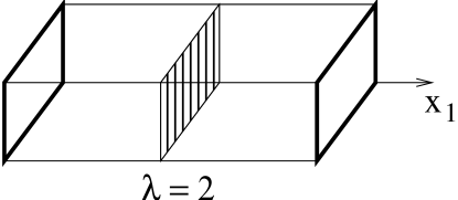
Figure 1: Basic plaquette moving operation.

This basic operation is successively performed in all directions. Note that, in $d$ dimensions, there are $(d-2)$ normal directions into which a plaquette can move. A plaquette moved to the $(d-1)$-dimensional cell boundary can still be moved in $(d-3)$ directions inside the cell boundary. The moving operation terminates when all plaquettes have been moved in this manner to form a tiling of the $2$-dimensional faces of a lattice of spacing $\lambda a$. The integrations over the bonds of the tiling plaquettes inside each such face can now be performed exactly (being $2$-dimensional), thus merging the tiling plaquettes into one plaquette of the coarse lattice of spacing $\lambda a$.

In terms of the definitions and notations introduced above, the end result can be concisely stated as follows. Under successive decimations

$$a\to\lambda a\to\lambda^{2}a\to\cdots\to\lambda^{n}a$$

$$\Lambda\to\Lambda^{(1)}\to\Lambda^{(2)}\to\cdots\to\Lambda^{(n)}$$

the resulting RG transformation rule is:

$$f(U,n-1)\to F_{0}(n)\,f(U,n)$$ (7)

with

$$f(U,n)=\Big{[}1+\sum_{j\not=0}\,d_{j}c_{j}(n)\,\chi_{j}(U)\Big{]}\;,$$ (8)

and

$$c_{j}(n)=\hat{c}_{j}(n)^{\lambda^{2}}\;,\qquad F_{0}(n)=\hat{F}_{0}(n)^{\lambda^{2}}\;,$$ (9)

where

$$\hat{c}_{j}(n)\equiv\hat{F}_{j}(n)/\hat{F}_{0}(n)\leq 1\;,\qquad j\not=0\;,$$ (10)

$$\hat{F}_{j}(n)=\int\,dU\;\Big{[}\,f(U,n-1)\,\Big{]}^{\zeta}\,{1\over d_{j}}\,\chi_{j}(U)\;,$$ (11)

The renormalization parameter $\zeta$ controls by how much the plaquettes remaining after each decimation step have been strengthened to compensate for the removed plaquettes. What has been considered in the literature almost exclusively is the choice $\zeta=\lambda^{(d-2)}$. This is essentially the original choice in [2], and will be referred to as the MK choice. Here we consider $\zeta$ an adjustable parameter.

The resulting partition function after $n$ decimation steps is:

$$Z_{\Lambda}(\beta,n) = \prod_{m=0}^{n}F_{0}(m)^{|\Lambda|/\lambda^{md}}$$ (12)

$$\cdot\;\int dU_{\Lambda^{(n)}}\;\prod_{p\in\Lambda^{(n)}}\,f_{p}(U,n)\;.$$

As a point of notation, the dependence of the quantities $F_{0}(n)$, $c_{j}(n)$, etc. on variables such as $\lambda$, $\zeta$, or the set of couplings $\beta$, which characterize the choice of decimation and action at the original spacing $a$, will not be indicated explicitly unless specific reference to it is required.

It is important to note that after each decimation step the resulting action retains the original one-plaquette form but will, in general, contain all representations:

$$A_{p}(U,n)=b_{0}(n)+\sum_{j\not=0}\;d_{j}\,\beta_{j}(n,\beta)\,\chi_{j}(U)\;.$$ (13)

Furthermore, among the effective couplings $\beta_{j}(n,\beta)$ some negative ones may in general occur. These features are present even after a single decimation step $a\to\lambda a$ starting with the usual single representation (fundamental) Wilson action.

Preservation of the one-plaquette form of the action is of course what makes these decimations simple to explore. The rule specified by (7)- (11) is meaningful for any real (positive) $\zeta$. Here, however, a basic distinction can be made. For integer $\zeta$, the important property of positivity of the Fourier coefficients in (1), (4):

$$F_{0}(n)\geq 0\quad,\qquad c_{j}(n)\geq 0\;,$$ (14)

and hence reflection positivity are maintained at each decimation step. This, in general, is not the case for non-integer $\zeta$. Thus non-integer $\zeta$ results in approximate RG transformations that violate the reflection positivity of the theory (assuming a reflection positive starting action). From now on we assume that (14) holds.

There are various other interesting features of such decimations. The following property, in particular, is important. One can show that, given the coefficients $c_{j}(n)$ after $n$ decimations, one has the general relation

$$\sum_{j}\;c_{j}(n)\,\Big{(}\,\hat{c}_{j}(n+1,\zeta)-c_{j}(n)\,\Big{)}\geq 0\;.$$ (15)

It follows from (15) that the ($l_{2}$) norm of the vector ${\bf\hat{c}}(n+1)$ formed from the $\hat{c}_{j}(n+1)$ coefficients is bigger than that of the vector of the $c_{j}(n)$:

$$||{\bf\hat{c}}(n+1)||_{2}\geq||{\bf c}(n)||_{2}\;.$$ (16)

All coefficients being positive, this implies that (15) must hold also component-wise, ie.

$$\hat{c}_{j}(n+1)\geq c_{j}(n)\;,$$ (17)

for at least a subset of components giving the dominant contribution to the norms. For $\zeta=1$, it follows immediately from (10) - (11) that (17) holds as an equality for all $j$. For general $\zeta$, one finds by explicit numerical evaluations that, in fact, (17) also holds for all $j$. This can be shown analytically in special cases and can probably be proved in general.

Alternatively, instead of attempting such a proof, one may impose (17) as part of the specification of the decimation transformation. This amounts to replacing (10) by

$$\hat{c}_{j}(n) = {\hat{F}_{j}(n)\over\hat{F}_{0}(n)}\;\Theta\Big{[}\,{\hat{F}_{j}(n)\over\hat{F}_{0}(n)}-c_{j}(n-1)\,\Big{]}$$ (18)

$$+ c_{j}(n-1)\;\Theta\Big{[}\,c_{j}(n-1)-{\hat{F}_{j}(n)\over\hat{F}_{0}(n)}\,\Big{]}.$$

3 The exact partition function

Since our decimations are not exact decimation transformations, the partition function does not in general remain invariant under them. The subsequent development hinges on the following two basic propositions that can now be proved:

(I) With $\zeta=\lambda^{d-2}$:

$$Z_{\Lambda}(\beta,n)\leq Z_{\Lambda}(\beta,n+1)\;.$$ (19)

(II) With $\zeta=1$:

$$Z_{\Lambda}(\beta,n+1)\leq Z_{\Lambda}(\beta,n)\;.$$ (20)

Note that for $d=2$ (19) - (20) express the well-known fact that the decimations become exact. For $d>2$, in both (I), (II) one in fact has strict inequality.

(I) says that modifying the couplings of the remaining plaquettes after decimation by taking $\zeta=\lambda^{d-2}$ (standard MK choice [2]) results into overcompensation (upper bound on the partition function). (II) says that decimating plaquettes while leaving the couplings of the remaining plaquettes unaffected results in a lower bound on the partition function. Translation invariance, convexity of the free energy and reflection positivity underlie (19).

Consider now the, say, $(n-1)$-th decimation step with Fourier coefficients $c_{j}(n-1)$, which we relabel $c_{j}(n-1)=\tilde{c}_{j}(n-1)$. Given these $\tilde{c}_{j}(n-1)$, we proceed to compute the coefficients $F_{0}(n)$, $c_{j}(n)$ of the next decimation step according to (7)-(11) above with $\zeta=\lambda^{d-2}$.

Then introducing a parameter $\alpha$, ($0\leq\alpha$), define the interpolating coefficients:

$$\tilde{c}_{j}(n,\alpha)=\tilde{c}_{j}(n-1)^{\lambda^{2}(1-\alpha)}\,c_{j}(n)^{\alpha}\,,$$ (21)

so that

$$\tilde{c}_{j}(n,\alpha)=\left\{\begin{array}[]{lll}c_{j}(n)&:&\alpha=1\\ \tilde{c}_{j}(n-1)^{\lambda^{2}}&:&\alpha=0\end{array}\right.$$ (22)

The $\alpha=0$ value is that of the $n$-th step coefficients resulting from (9)-(11) with $\zeta=1$.

Thus defining the corresponding partition function

$$Z_{\Lambda}(\beta,\alpha,n) = \big{(}\prod_{m=0}^{n-1}F_{0}(m)^{|\Lambda|/\lambda^{md}}\big{)}\;F_{0}(n)^{\alpha}$$ (23)

$$\cdot\>\int dU_{\Lambda^{(n)}}\!\!\prod_{p\in\Lambda^{(n)}}f_{p}(U,n,\alpha)$$

where

$$f_{p}(U,n,\alpha)=\Big{[}1+\sum_{j\not=0}d_{j}\,\tilde{c}_{j}(n,\alpha)\,\chi_{j}(U)\Big{]}\,,$$ (24)

we have from (19), (20)), and (22) above:

$$Z_{\Lambda}(\beta,0,n)\leq Z_{\Lambda}(\beta,n-1)\leq Z_{\Lambda}(\beta,1,n)\;.$$ (25)

Now the partition function (23) is a continuous in $\alpha$. So (25) implies that, by continuity, there exist a value of $\alpha$:

$$\alpha=\alpha^{(n)}(\beta,\lambda,\Lambda)\,,\qquad 0<\alpha^{(n)}(\beta,\lambda,\Lambda)<1$$

such that

$$Z_{\Lambda}(\beta,\alpha^{(n)},n)=Z_{\Lambda}(\beta,n-1)\;.$$ (26)

In other words there is an $\alpha$ at which the $n$-th decimation step partition function equals that obtained at the previous decimation step; the partition function does not change its value under the decimation step $\lambda^{n-1}a\to\lambda^{n}a$.

So starting at original spacing $a$, at every decimation step $m$, ($m=0,1,\cdots,n$), there exist a value $0<\alpha^{(m)}<1$ such that

$$Z_{\Lambda}(\beta,\alpha^{(m+1)},m+1)=Z_{\Lambda}(\beta,\alpha^{(m)},m)\,.$$ (27)

This then gives, after $n$ successive decimations, a representation of the exact partition function in the form:

$$Z_{\Lambda}(\beta) = F_{0}^{|\Lambda|}\;\int dU_{\Lambda}\;\prod_{p\in\Lambda}\,f_{p}(U,a)$$ (28)

$$= \prod_{m=0}^{n}F_{0}(m)^{\alpha^{(m)}|\Lambda|/\lambda^{md}}\;$$

$$\cdot\;Z_{\Lambda^{(n)}}(\beta,n,\alpha^{(n)}),$$

where

$$Z_{\Lambda^{(n)}}(\beta,n,\alpha^{(n)}) \equiv \int dU_{\Lambda^{(n)}}\;$$ (29)

$$\cdot\;\prod_{p\in\Lambda^{(n)}}\,f_{p}(U,n,\alpha^{(n)}),$$

i.e. a representation in terms of the successive bulk free energy contributions from the $a\to\lambda\to\cdots\to\lambda^{n}a$ decimations and a one-plaquette effective action on the resulting lattice $\Lambda^{(n)}$.

At weak and strong coupling $\alpha^{(m)}$ may be estimated analytically. At large $\beta$, where the decimations approximate the free energy rather accurately, the appropriate $\alpha$ values are very close to unity. At strong coupling they may be estimated by comparison with the strong coupling expansion. On any finite lattice there is also a weak volume dependence as a correction which goes away as an inverse power of the lattice size.

For most purposes the exact values of the $\alpha^{(m)}$’s, beyond the fact that are fixed between $0$ and $1$, are not immediately relevant. The main point of the representation (28) is that it can in principle relate the behavior of the exact theory to that of the easily computable approximate decimations.

Indeed, starting from the $\tilde{c}_{j}(n-1,\alpha^{(n-1)})$’s at the $(n-1)$-th step, consider the coefficients at the next step, and compare those evaluated at $\alpha=\alpha^{(n)}$, i.e.  $\tilde{c}_{j}(n,\alpha=\alpha^{(n)})$, to those evaluated at $\alpha=1$, i.e  $\tilde{c}_{j}(n,\alpha=1)\equiv c_{j}(n)$. The latter will be referred to as the MK coefficients. (Recall that $\alpha=1\Longleftrightarrow\zeta=\lambda^{d-2}$, the standard MK choice. The absence of a tilde on a coefficient in the following always means that it is computed at $\alpha=1$.) According to (I), the MK coefficients give an upper bound.

Now, (21) implies that

$$\tilde{c}_{j}(n,\alpha)\leq(1-\alpha)\,\tilde{c}_{j}(n-1)^{\lambda^{2}}+\alpha\,c_{j}(n)\,,$$ (30)

from which, by property (17), one has

$$\tilde{c}_{j}(n,\alpha)\leq c_{j}(n)\qquad\mbox{for {\it any}}\quad 0\leq\alpha\leq 1\;.$$ (31)

This has the following important consequence.

(31) says that the Fourier coefficients of the representation (28) are bounded from above by the MK coefficients ($\alpha=1$). Thus, if the $c_{j}(n)$’s are non-increasing, so are the $\tilde{c}_{j}(n,\alpha)$. The $c_{j}(n)$’s must then approach a fixed point, and hence so must the $\tilde{c}_{j}(n,\alpha)$’s, since $c_{j}(n),\tilde{c}_{j}(n,\alpha)\geq 0$. Note the fact that this conclusion is independent of the specific value of the $\alpha$’s at every decimation step.

In particular, if the $c_{j}(n)$’s approach the strong coupling fixed point, i.e. $F_{0}\to 1$, $c_{j}(n)\to 0$ as $n\to\infty$, so must the $\tilde{c}_{j}(n,\alpha)$’s of the exact representation. If the MK decimation coefficients flow to the confining regime, so do those in the exact representation (28). As it is well-known by explicit numerical evaluation, the MK decimations for $SU(2)$ and $SU(3)$ indeed flow to the strong coupling confining regime for all $\beta<\infty$ and $d\leq 4$. Above the critical dimension $d=4$, the decimations result in free spin wave behavior.

What do these results imply about the question of confinement in the exact theory? Though strongly suggestive, the fact that the long distance part, $Z_{\Lambda^{(n)}}$, in (28) flows in the confining regime does not suffice to answer the question. It is the combined contributions from all scales in (28) that combine to give one bulk quantity, the exact free energy $-\ln Z_{\Lambda}(\beta)$. As it is well-known, it is not possible to unambiguously determine the long distance behavior of the theory from that of a bulk quantity like the free energy. For that one needs to consider appropriate long distance order parameters.

4 Order parameters - Vortex free energy

The above derivation leading to the representation (28) for the partition function cannot be applied in the presence of observables without modification. Thus, in the presence of operators involving external sources, such as the Wilson or ’t Hooft loop, translation invariance is lost. Reflection positivity is also reduced to hold only in the plane bisecting the loop. Fortunately, there are other order parameters that can characterize the possible phases of the theory while maintaining translational invariance. They are the well-known vortex free energy, and its $Z(N)$ Fourier transform (electric flux free energy). They are in fact the natural order parameters in the present context since they are constructed out of partition functions. Recall that the vortex free energy is defined by

$$e^{-F_{v}(\tau)}=Z_{\Lambda}(\tau)/Z_{\Lambda}\;.$$ (32)

Here $Z_{\Lambda}(\tau)$ denotes the partition function with action modified by the ‘twist’ $\tau\in Z(N)$ for every plaquette on a coclosed set of plaquettes ${\cal V}$ winding through the periodic lattice in $(d-2)$ directions, i.e. through every $[\mu\nu]$-plane for fixed $\mu,\nu$:

$$A_{p}(U_{p})\to A_{p}(\tau U_{p})\;,\qquad\mbox{if}\quad p\in{\cal V}\;.$$

One has $Z_{\Lambda}(1)=Z_{\Lambda}$. A nontrivial twist ($\tau\not=1$) represents a discontinuous gauge transformation on the set ${\cal V}$ which introduces $\pi_{1}(SU(N)/Z(N))$ vortex flux rendered topologically stable by being wrapped around the lattice torus. As indicated by the notation, $Z_{\Lambda}(\tau)$ depends only on the presence of the flux, and is invariant under changes in the exact location of ${\cal V}$. The vortex free energy is then the ratio of the partition function in the presence of this external flux to the partition function in the absence of the flux (the latter is what was considered above). As it is well-known the possible phases of a gauge theory (Higgs, Coulomb, confining) can be characterized by the behavior of (32). Furthermore, by rigorous correlation inequalities [4], the Wilson loop, Wilson line correlators, and the ’t Hooft loop can in turn be bounded by the vortex free energy and its $Z(N)$ Fourier transform. For $SU(2)$ the only nontrivial element is $\tau=-1$.

The above development, in particular the derivation of (28), should then be repeated for $Z_{\Lambda}(-1)\equiv Z_{\Lambda}^{(-)}$. There is, however, a technical complication in obtaining the analog to (28) for $Z_{\Lambda}^{(-)}$. The presence of the flux reduces reflection positivity to hold only in planes perpendicular to the directions in which the flux winds through the lattice. This may be circumvented by considering $Z_{\Lambda}+Z_{\Lambda}^{(-)}$ instead of $Z_{\Lambda}^{(-)}$. Indeed, for $Z_{\Lambda}+Z_{\Lambda}^{(-1)}$ reflection positivity is easily checked to again hold in all planes. The proof of propositions (I) and (II), and the subsequent derivation leading to (27), and (28) can then be carried through for the quantity $Z_{\Lambda}+Z_{\Lambda}^{(-)}$ to obtain

$$Z_{\Lambda}(\beta)+Z_{\Lambda}^{(-)}(\beta)=\prod_{m=0}^{n}F_{0}(m)^{\alpha^{(m)}|\Lambda|/\lambda^{md}}$$

$$\qquad\cdot\;\Big{(}\,Z_{\Lambda^{(n)}}(\beta,n,\alpha^{(n)})+Z^{(-)}_{\Lambda^{(n)}}(\beta,n,\alpha^{(n)})\,\Big{)}$$ (33)

where

$$Z^{(-)}_{\Lambda^{(n)}}=\int dU_{\Lambda^{(n)}}\prod_{{p\notin{\cal V}\atop p\in\Lambda^{(n)}}}\,f_{p}(U,n,\alpha^{(n)})$$

$$\qquad\qquad\cdot\;\prod_{{p\in{\cal V}\atop p\in\Lambda^{(n)}}}\,f_{p}((-1)U,n,\alpha^{(n)})\,\big{)}.$$ (34)

The values $\{\alpha^{(m)}\}$ in (33), as fixed by the interpolating argument between the upper and lower bounds for the quantity $Z_{\Lambda}+Z_{\Lambda}^{(-)}$, are a priori distinct from those in (28) fixed by the analogous argument for the quantity $Z_{\Lambda}$. It is not hard to see, however, that in fact they have to coincide for large lattices.

Using (28) and (33) in (32) then gives for the vortex free energy:

$$e^{-F_{v}(\tau)}={Z^{(-)}_{\Lambda^{(n)}}(\beta,n,\alpha^{(n)})\over Z_{\Lambda^{(n)}}(\beta,n,\alpha^{(n)})}\;.$$ (35)

It manifestly couples only to the long distance part as it should. Bulk (local) free energy contributions resulting from each successive decimation are unaffected by the presence of the flux and cancel. By our previous considerations, the strategycoefficients $\tilde{c}_{j}(n,\alpha^{(n)})$ occurring in $Z_{\Lambda^{(n)}}$, $Z^{(-)}_{\Lambda^{(n)}}$ in (35) are bounded (regardless of the specific values of the $\alpha^{(n)}$ parameters) by the corresponding MK coefficients $c_{j}(n)\equiv\tilde{c}_{j}(n,\alpha=1)$. By taking $n$ large enough, the latter tend to zero no matter how large the initial $\beta$ is chosen. Thus taking $n$ large enough to enter the strong coupling regime, (35) can be evaluated exactly within the convergent strong coupling cluster expansion in terms of the $\tilde{c}_{j}(n,\alpha^{(n)})$’s by standard computations. The vortex free energy is thus explicitly shown to exhibit confining behavior. This, by the known inequalities [4] relating the vortex free energy to the Wilson loop, then also necessarily implies area law for the latter.

An expanded account with the proofs of (I), (II) and various other statements above will appear elsewhere.

I am grateful to the organizers of the QCD Down Under Workshop for organizing such a stimulating meeting in a thoroughly enjoyable environment in Adelaide and the Barossa Valley, and to the participants for a great many discussions.

References

- [1] J. Greensite, Progr. Part. Nucl. Phys. 51 (2003) 1, (hep-lat/0301023).
- [2] A. A. Migdal, Sov. Phys. JETP 42 (1976) 413, 743; L. Kadanoff, Ann. Phys. (N.Y.) 100 (1976) 369.
- [3] M. Nauenberg and D. Toussaint, Nucl. Phys. B190 [FS3] (1981) 217; K. Bitar, S. Gottlieb and C. Zachos, Phys. Rev. D26 (1982) 2853.
- [4] E. T. Tomboulis and L. G. Yaffe, Comm. Math. Phys. 100 (1985) 313; T. G. Kovács and E. T. Tomboulis, Phys. Rev. D26 (2002) 074501 (hep-lat/0108017).