Extracting excited states from lattice QCD: the Roper resonance

Abstract

We present a new method for extracting excited states from a single two-point correlation function calculated on the lattice. Our method simply combines the correlation function evaluated at different time slices so as to “subtract” the leading exponential decay (ground state) and to give access to the first excited state. The method is applied to a quenched lattice study (volume = $24^{3}\times 64$, $\beta=6.2$, $a^{-1}=2.55$ GeV) of the first excited state of the nucleon using the local interpolating operator $\mathcal{O}=\varepsilon_{abc}[u^{T}_{a}C\gamma_{5}d_{b}]u_{c}$. The results are consistent with the identification of our extracted excited state with the Roper resonance $N^{\prime}(1440)$. The switching of the level ordering with respect to the negative-parity partner of the nucleon, $N^{*}(1535)$, is not seen at the simulated quark masses and, basing on crude extrapolations, is tentatively expected to occur close to the physical point.

1 Introduction

Hadron spectroscopy offers a well defined framework to test the non-perturbative regime of QCD and to shed light on the mechanism responsible for confinement. Of course, the masses of ground states do not offer sufficient information to unravel the dynamics responsible for that mechanism, but fundamental insight can be gained by accessing the masses of excited states as well.

As is well known, one of the long-standing puzzles in baryon spectroscopy is the level ordering between the negative-parity partner of the nucleon, $N^{*}(1535)$, and the first excitation of the nucleon, the so-called Roper resonance $N^{\prime}(1440)$. Phenomenological low-energy models of QCD are generally quite successful in explaining many features of baryon mass spectra Capstick . Some of them are however unable to explain the proper level ordering between positive- and negative-parity excited states of the nucleon, like e.g. the one-gluon-exchange quark model of Ref. Isgur ; such a failure has led to the speculation that the Roper resonance cannot be described by a picture based only on three constituent quarks. Other models do reproduce the correct level ordering, like the Goldstone-boson-exchange quark model of Ref. Glozman , where the level switching between the radial and orbital excitations of the nucleon is a consequence of the spontaneous breaking of chiral symmetry.

It is clear that a non-perturbative approach based on first principles, such as lattice QCD, offers a unique possibility to unfold the above issues and, in particular, to investigate the evolution of the excitations of the nucleon as a function of the quark masses. Ground-state spectroscopy in lattice QCD is well established and there is a general agreement with experimental data at the level of $5\div 10\%$ precision ground . On the contrary it is still challenging to measure the mass of an excited state. Both ground and excited masses are extracted from the (Euclidean) time behavior of two-point correlators and therefore a clean separation among them is required. This problem is currently addressed following two main approaches.

The first approach uses a single two-point correlator, constructed from an interpolating field with appropriate quantum numbers. A naive multiple-exponential fit of the time dependence of the latter is in general affected by large systematic or statistical errors, due to the contamination from high excited states and/or to the large number of fitting parameters. To circumvent this problem, methods inspired by Bayesian statistics, like the constrained curve fitting method lepage or the maximum entropy method mem , were developed and applied to lattice analyses aimed at studying the Roper resonance dong ; sasaki . The crucial point of these methods is clearly the choice of the priors (see Ref. priors ).

The second approach uses several two-point correlators constructed from various interpolating operators $\mathcal{O}_{i}$ which couple differently to the states of interest variational . A matrix of correlation functions is constructed choosing in all possible (independent) ways the source and the sink operators. By solving an appropriate eigenvalue problem, the contributions coming from the various states coupled to the operators $\mathcal{O}_{i}$ are disentangled, so that the masses of ground and excited states can be determined from the eigenvalues (see Refs. UKQCD ; leinweber ). The interpolating operators must be chosen properly, taking into account the computational cost of constructing a matrix of correlators. The following two (local) operators are commonly employed leinweber ; sbo ; bgr1 :

$$\mathcal{O}(x)=\varepsilon_{abc}[u^{T}_{a}C\gamma_{5}d_{b}]u_{c}(x)~{},$$

$$\mathcal{O}^{\prime}(x)=\varepsilon_{abc}[u^{T}_{a}Cd_{b}]\gamma_{5}u_{c}(x)~{},$$ (1.1)

where $C$ is the charge conjugation Dirac matrix. It is known richards that the first and the second operators in Eq. (1.1) are, respectively, strongly and very weakly coupled to the ground state of the nucleon. A recent improvement bgr2 is the use of different smeared interpolating operators as a tool to generate nodes in the radial wave function, which allows to capture more efficiently the Roper signal. The crucial point of the “matrix” approach is a careful choice of the time interval, where the correlator matrix of dimension $N$ has to be dominated by the first $N$ states.

We point out that a precise determination of excited states on the lattice is computationally very demanding on its own, since the size and the mass of the state increases with the excitation, which in turn implies the use of large lattice volumes and fine lattice spacings in order to keep under control systematic errors (see Ref. sasaki ).

In this paper we show that it is possible to access the first excited state coupled to a single two-point correlator $G(t)$, defining a new correlator which is simply an appropriate combination of $G(t)$ taken at different time slices. The mass of the first excited state can be extracted from the plateau of the effective mass of the new correlator. Therefore our method allows to establish unambiguously the time interval where the ground and the first excited states dominate the two-point correlator $G(t)$. In this way no prior is needed at all and the extracted resonance mass is not affected by contaminations from higher excited states.

Our procedure is explained in Section 2, while its application to the extraction of the Roper mass, using the local interpolating field $\mathcal{O}$, is presented in Section 3. In Section 4 we draw our conclusions and outlook.

2 The method

We limit ourselves to consider a single local operator which has a good overlap with both positive- and negative-parity baryon states, i.e.

$$\mathcal{O}_{\gamma}(x)=\varepsilon_{abc}[u^{T}_{a}C\gamma_{5}d_{b}]~{}u_{c\gamma}(x)~{},$$ (2.2)

where Latin indices denote color and Greek indices refer to the Dirac structure, that is contracted in the (ud) diquark on the r.h.s. of Eq. (2.2). Let us then define in the usual way the two-point (zero-momentum) correlation function for the operator (2.2) as

$$G_{\gamma^{\prime}\gamma}(t)=\sum_{\mathbf{x}}\langle 0|T\left\{\mathcal{O}_{\gamma^{\prime}}(\mathbf{x},t)\bar{\mathcal{O}}_{\gamma}(\mathbf{0},0)\right\}|0\rangle~{}.$$ (2.3)

Adopting periodic boundary conditions on the lattice, Eq. (2.3) can be expanded as

$$G(t) = \left(\frac{1+\gamma_{4}}{2}\right)\sum_{i\geq 0}\left(Z_{i}^{+}e^{-aM_{i}^{+}t}-Z_{i}^{-}e^{-aM_{i}^{-}(T-t)}\right)$$

$$+ \left(\frac{1-\gamma_{4}}{2}\right)\sum_{i\geq 0}\left(Z_{i}^{+}e^{-aM_{i}^{+}(T-t)}-Z_{i}^{-}e^{-aM_{i}^{-}t}\right),$$

where $t$ is an integer number in units of the lattice spacing $a$, $T$ represents the time extension of the lattice, the suffixes $\pm$ refer to the positive- and negative-parity states coupled to (2.2), respectively, $M_{i}^{\pm}$ refers to the masses of the given-parity tower of states, and $Z_{i}^{\pm}$ are the corresponding couplings with the interpolating operator.

Choosing $\gamma_{4}$ diagonal, one gets

$$G(t) \equiv {1\over 4}\left[G_{11}(t)+G_{22}(t)+G_{33}(T-t)+G_{44}(T-t)\right]$$ (2.5)

$$= \sum_{i\geq 0}\left[Z_{i}^{+}e^{-aM_{i}^{+}t}-Z_{i}^{-}e^{-aM_{i}^{-}(T-t)}\right]$$

Assuming ($T-t$) sufficiently large one has

$$G(t)=\sum_{i\geq 0}Z_{i}^{+}~{}e^{-aM_{i}^{+}t}$$ (2.6)

from which the mass of the positive-parity ground state can be extracted from the large-time behavior through an effective mass analysis.

Let us define the following quantity

$$\widehat{G}(t)\equiv G(t+1)G(t-1)-G^{2}(t)~{},$$ (2.7)

which, by direct substitution of Eq. (2.6), can be expanded as

$$\widehat{G}(t) = 2\sum_{j>i=0}^{\infty}Z_{i}^{+}Z_{j}^{+}e^{-(aM_{i}^{+}+aM_{j}^{+})t}$$ (2.8)

$$\cdot \left[\cosh(aM_{j}^{+}-aM_{i}^{+})-1\right]~{}.$$

One immediately sees that the diagonal terms $i=j$ are cancelled out in the new correlator and that the leading exponential decay in Eq. (2.8) is governed by the sum of the masses of the first two states $aM_{0}^{+}$ and $aM_{1}^{+}$. Thus, an effective mass analysis applied to $\widehat{G}(t)$ provides the quantity $a(M_{0}^{+}+M_{1}^{+})$. The use of the “modified” correlator (2.8) is expected to work when the mass gap between the ground state and the first excited state is sufficiently large, since for a small mass gap the factor $[\cosh(aM_{1}^{+}-aM_{0}^{+})-1]$, which multiplies the exponential in the r.h.s. of Eq. (2.8), suppresses the signal.

One can thus set up the following general procedure for extracting the first excited state from correlators like (2.6):

• Extract the mass of the ground state $aM_{0}^{+}$ from the plateau of the effective mass for the correlator (2.6). Let the plateau region be given by the time interval $[t_{i},t_{f}]$.

• Extract the sum of the masses of the first two states, $a(M_{0}^{+}+M_{1}^{+})$, from the plateau of the effective mass for the“modified” correlator (2.7). Let the plateau region be the time interval $[t^{*}_{i},t^{*}_{f}]$. This second plateau is always such that $[t^{*}_{i},t^{*}_{f}]<[t_{i},t_{f}]$. Indeed, in the time interval $[t_{i},t_{f}]$ the correlator (2.6) is dominated by the ground state signal and the modified correlator (2.7) is pure noise, whereas in the time interval $[t^{*}_{i},t^{*}_{f}]$ the signal associated to the first excited state is visible in both correlators. This in turn means that in the larger time interval $[t^{*}_{i},t_{f}]$ the correlator (2.6) is dominated by the first two terms due to the ground and the first excited states, while the contribution from higher excited states is negligible, i.e. within statistical fluctuations.

• Check the consistency of the results obtained from i) and ii) for $aM_{0}^{+}$ and $aM_{1}^{+}$ with those coming from a double-exponential fit of the correlator (2.6) in the time interval from $t^{*}_{i}$ to $t_{f}$.

Note that one could in principle consider the modified propagator $\widehat{G}(t)$ divided by $G^{2}(t)$, because such a ratio may directly provide the mass difference $a(M_{1}^{+}-M_{0}^{+})$. However the leading exponential decays in $\widehat{G}(t)$ and $G^{2}(t)$ occur in different time intervals, as we will illustrate later, causing a mismatch between the plateau of the effective mass of the numerator and the one of the denominator.

In the next Section we apply our method to the extraction of the first excited state from the correlator (2.6), and we show that our extracted state can be reasonably identified with the Roper resonance.

3 Lattice study of the Roper mass

We have adopted Wilson fermions with non-perturbative Clover improvement and we have generated 450 quenched gauge configurations at $\beta=6.20$ in a lattice volume of $24^{3}\times 64$. The hopping parameter is assigned the following values: $k\in\{0.1352,0.1347,0.1342,0.1337,0.1332\}$. The analysis of pseudoscalar (PS) and vector meson masses yields a critical hopping parameter equal to $k_{c}=0.13588(2)$ and an inverse lattice spacing given by $a^{-1}=2.55(3)$ GeV. Note that our lattice spacing is significantly smaller than the ones adopted in Refs. dong ; sasaki ; leinweber ; sbo ; bgr1 ; bgr2 . The statistical errors for all the quantities considered in this work are evaluated using the jacknife grouping procedure jacknife . The values of the bare quark mass $m_{q}\equiv(1/k-1/k_{c})/2a$ and of the PS meson mass are: $m_{q}\in\{47,82,117,153,189\}$ MeV and $M_{PS}\in\{0.513,0.686,0.831,0.960,1.08\}$ GeV.

3.1 Determination of the positive-parity masses

The masses of the ground and first excited positive-parity states can be obtained from the correlators $G(t)$ [Eq. (2.6)] and $\widehat{G}(t)$ [Eq. (2.8)]. The ground state mass is extracted in a standard way by determining the plateau of the effective mass function corresponding to the correlator $G(t)$

$$aM_{eff}(t)=\ln\left\{G(t)/G(t+1)\right\}~{}.$$ (3.9)

Such a mass is identified with that of the nucleon, and in the following indicated with $aM_{N}$.

The sum of the masses $aM_{N}+aM_{N^{\prime}}$ of the ground and first excited states is correspondingly obtained from the plateau of the effective mass function related to the correlator $\widehat{G}(t)$

$$a\widehat{M}_{eff}(t)=\ln\left\{\widehat{G}(t)/\widehat{G}(t+1)\right\}~{}.$$ (3.10)

The quality of the plateaux for $aM_{eff}(t)$ and $a\widehat{M}_{eff}(t)$ is illustrated in Fig. 1.

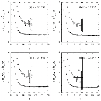
Fig. 1: Plateaux of the effective mass functions (3.9) (diamonds) and (3.10) (dots) for $k\in\{0.1332,0.1337,0.1342,0.1347\}$. The solid lines are the time extensions considered for the plateaux of Eqs. (3.9) and (3.10)

In Table 1 we report the mass values $aM_{N}$ and $aM_{N^{\prime}}$ obtained from the plateaux of Eqs. (3.9) and (3.10), respectively, at the different values of the hopping parameter used in the simulations. The time regions of the plateaux are reported in Table 1 and explicitly shown in Fig. 1 by the solid lines. Notice that the plateaux of Eq. (3.10) are of comparable extension with respect to those of the ground state effective mass, Eq (3.9).

$k$	$\begin{array}[]{c}t^{*}_{i}~{}-~{}t^{*}_{f}\\ t_{i}~{}-~{}t_{f}\end{array}$	$\begin{array}[]{c}aM_{N^{\prime}}\\ aM_{N}\end{array}$	$M_{N^{\prime}}/M_{N}$
$0.1332$	$\begin{array}[]{c}10~{}-~{}17\\ 20~{}-~{}30\end{array}$	$\begin{array}[]{c}1.189\pm 0.0181\\ 0.7534\pm 0.0027\end{array}$	$1.578\pm 0.025$
$0.1337$	$\begin{array}[]{c}10~{}-~{}17\\ 20~{}-~{}30\end{array}$	$\begin{array}[]{c}1.132\pm 0.022\\ 0.6911\pm 0.0033\end{array}$	$1.638\pm 0.034$
$0.1342$	$\begin{array}[]{c}10~{}-~{}17\\ 20~{}-~{}30\end{array}$	$\begin{array}[]{c}1.067\pm 0.031\\ 0.6262\pm 0.0042\end{array}$	$1.705\pm 0.052$
$0.1347$	$\begin{array}[]{c}10~{}-~{}17\\ 20~{}-~{}28\end{array}$	$\begin{array}[]{c}0.969\pm 0.039\\ 0.5561\pm 0.0058\end{array}$	$1.743\pm 0.075$
$0.1352$	$\begin{array}[]{c}10~{}-~{}17\\ 20~{}-~{}28\end{array}$	$\begin{array}[]{c}0.825\pm 0.053\\ 0.4832\pm 0.0054\end{array}$	$1.71\pm 0.11$

Table 1: Effective masses $aM_{N}$ and $aM_{N^{\prime}}$ at the different values of $k$ used in the simulations. The second column reports the time extensions of the plateaux of Eqs. (3.9) and (3.10).

To check the consistency of our results, we have then performed a double-exponential fit of the correlator (2.6) in the time coordinate, limiting the fitting region to the one including the plateaux of the two effective mass analyses, i.e. $[t^{*}_{i},t_{f}]$. In this fit we have considered two options for the nucleon mass $aM_{N}$: a) a free parameter to be fixed by the fitting procedure; b) a parameter fixed at the value obtained from the effective mass analysis of Eq. (3.9) [see the third column of Table 1]. The two options provide consistent results for both $aM_{N}$ and $aM_{N^{\prime}}$, but the uncertainties are definitely smaller in the case b). Our results for $aM_{N^{\prime}}$, corresponding to the latter option, are reported in Table 2. The consistency between the results of the effective mass analysis and the double-exponential fit can be appreciated from Fig. 2, where it can be seen that the more precise results are those obtained from the effective mass analysis.

$k$	$t^{*}_{i}~{}-~{}t_{f}$	$aM_{N^{\prime}}$
$0.1332$	$10~{}-~{}30$	$1.154\pm 0.033$
$0.1337$	$10~{}-~{}30$	$1.111\pm 0.047$
$0.1342$	$10~{}-~{}30$	$1.076\pm 0.074$
$0.1347$	$10~{}-~{}28$	$1.02\pm 0.11$
$0.1352$	$10~{}-~{}28$	–

Table 2: Results for the mass of the first excited positive-parity state obtained from a double-exponential fit of the correlator (2.6) in the time region $[t_{i}^{*},t_{f}]$ which includes the plateaux of the effective masses (3.9) and (3.10). In this fit the nucleon mass $aM_{N}$ is constrained to be the one obtained from the effective mass analysis (3.9).

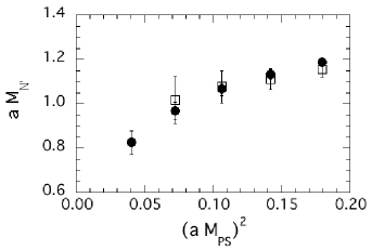
Fig. 2: Comparison of the mass of the first excited positive-parity state, $aM_{N^{\prime}}$, obtained for different quark masses using the effective mass method (full dots) and the double-exponential fit (open squares).

3.2 Determination of the negative-parity mass $M_{N^{*}}$

The analysis of the negative-parity ground state of the correlator (2.6) strictly follows that of the positive-parity one, described in the previous subsection. One simply has to consider $t$ sufficiently large so that Eq. (2.6) can be replaced by

$$G(t)=-\sum_{i\geq 0}Z_{i}^{-}~{}e^{-aM_{i}^{-}(T-t)}$$ (3.11)

$k$	$(T-t)_{i}~{}-~{}(T-t)_{f}$	$aM_{N^{*}}$
$0.1332$	$14~{}-~{}19$	$0.926\pm 0.009$
$0.1337$	$14~{}-~{}19$	$0.860\pm 0.011$
$0.1342$	$14~{}-~{}19$	$0.791\pm 0.015$
$0.1347$	$14~{}-~{}19$	$0.717\pm 0.023$
$0.1352$	$12~{}-~{}17$	$0.697\pm 0.026$

Table 3: Results for the negative-parity ground-state mass $aM_{N^{*}}$ obtained through the effective mass analysis (3.9). The time intervals of the plateaux are also reported.

In Table 3 we report the values obtained for $aM_{N^{*}}$ from the effective mass analysis of the correlator (3.11), together with the corresponding time intervals for the plateaux. The latter are shown in Fig. 3 for a couple of values of the quark mass. It can be seen that the ground-state signal is of good quality, but with respect to the case of positive-parity the plateaux are narrower and shifted to lower values of the lattice time, mainly because of the higher mass of the negative-parity ground state.

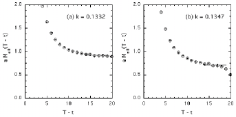
Fig. 3: Plateaux of the effective mass function (3.9) for the (negative-parity) correlator (3.11) for $k=0.1332$ (a) and $k=0.1347$ (b).

In Fig. 4 our results for $aM_{N^{*}}$ are plotted versus the squared PS mass $(aM_{PS})^{2}$. As a consistency check, we have performed a single-exponential fit of the correlator (3.11) in the time interval corresponding to the plateaux reported in Table 3. The results are shown in Fig. 4 as open squares.

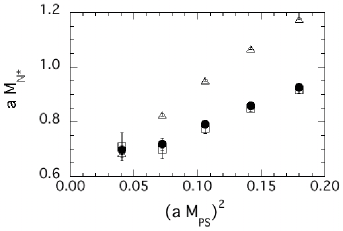
Fig. 4: Results obtained for $aM_{N^{*}}$ from the effective mass analysis (full dots) and from a single-exponential fit in the time interval (open squares) versus the square of the PS mass. The sum of the masses $aM_{N}+aM_{PS}$ (open triangles) is also plotted for comparison.

Our lattice simulations can be directly compared with those of Ref. goeckeler , since the only difference is the use of smeared interpolating operators in the latter. The two simulations nicely agree in the results for both $aM_{N}$ and $aM_{N^{*}}$.

In Fig. 4 the mass $aM_{N}+aM_{PS}$ of the (S-wave) scattering state $N+PS$ at zero hadron momenta, is reported for comparison. Note that such a scattering state stays higher in energy with respect to the resonance state for the quark masses used in the present simulations, except for the lightest mass where they nearly coincide (cf. also Ref. goeckeler ). In principle the mass of the scattering state can be extracted using the modified correlator (2.8) constructed as in Eq. (2.7) from the negative-parity propagator (3.11). However in practice, due to the occurrence of the plateaux of the negative-parity ground-state at quite earlier times compared with the case of the positive-parity one (see Tables 1 and 3), as well as to a smaller mass gap and to larger statistical fluctuations, we find no clear signal of the scattering state $N+PS$ in the modified correlator.

Though it is beyond the aim of the present study, we want to briefly comment on the systematic errors of our simulations before closing the subsection.

Our calculations have been carried out at a fixed value of the lattice spacing $a$. The use of the non-perturbative Clover improvement guarantees that discretization errors of order $\mathcal{O}(a)$ are absent in our extracted masses. Nevertheless the closeness to the continuum limit strongly depends on the condition $aM\ll 1$, which is better fulfilled by our results for the positive-parity ground-state (the nucleon). In case of $aM_{N^{*}}$ and $aM_{N^{\prime}}$ the discretization error should be investigated by performing simulations at different values of the lattice spacing. In this respect we point out again that the value of $a$ employed in our study is much lower than those used in most of the works appeared in the literature on the subject, like Refs. dong ; sasaki ; leinweber ; sbo ; bgr1 ; bgr2 .

As shown in sasaki , finite volume effects can affect the extracted mass of excited states. The estimates made in sasaki indicate that at the volume and the quark masses used in our lattice simulations one can expect a $\approx 10\div 20\%$ reduction of the resonance masses.

Finally, the error due to the quenched approximation can be estimated only by removing such approximation. Available results in the literature ground suggest that the quenching error on the ground-sate baryon spectrum is not large and expected within $\approx 10\%$. However, very little is known about the impact of the quenched approximation on the excited baryon spectrum.

3.3 Extrapolation to the physical point

All our lattice results for $aM_{N}$, $aM_{N^{*}}$ and $aM_{N^{\prime}}$ are shown in Fig. 5 versus the square of the PS mass. Up to the lightest quark mass used in our simulations there is no level switching between the negative-parity ground-state and the positive-parity first excited state, the latter lying above the former at variance with the physical spectrum.

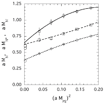
Fig. 5: Plot of $aM_{N}$ (diamonds), $aM_{N^{*}}$ (squares) and $aM_{N^{\prime}}$ (dots) versus the square of the PS mass. The dotted, dashed and solid lines are analytical fits of the form $A+B(aM_{PS})^{2}+C(aM_{PS})^{4}$. The markers at the physical point correspond in lattice units to the physical masses of the nucleon N(938), the $S_{11}(1535)$ and $N^{\prime}(1440)$ resonances.

The extrapolation to the physical point should be guided by chiral perturbation theory. However, the quark masses used in our simulations are quite far from the chiral regime and indeed we expect that the results shown in Fig. 5 do not contain sizable effects from chiral logs. In order to identify the masses found on the lattice with the resonances of the physical spectrum, one should perform simulations at lower quark masses. For a naïve correspondence we will limit ourselves to adopt an analytical quark mass dependence of the form $aM=A+B(aM_{PS})^{2}+C(aM_{PS})^{4}$, which is represented by the lines in Fig. 5 for the various states. The positive- and negative-parity ground states can be reasonably identified with nucleon $N(938)$ and the $S_{11}(1535)$ resonance. As for the positive-parity first excited state, the quark mass dependence of our extracted masses is consistent with the identification with the Roper resonance $N^{\prime}(1440)$, though a possible interpretation as the higher nucleon resonance $N(1710)$ cannot be completely ruled out. Such a possible extrapolation ambiguity is not addressed in the literature dong ; sasaki ; leinweber ; sbo ; bgr1 , and a clear-cut solution again relies in performing lattice simulations at lower quark masses. The latter would also help clarifying at which quark masses the level switching between the orbital and radial excitations of the nucleon occurs. Basing on our crude extrapolations such a crossing is tentatively expected to appear close to the physical point.

4 Conclusions

We have presented a new method for extracting excited states from a single two-point correlation function calculated on the lattice. We have defined a new correlator which is simply an appropriate combination of the correlation function evaluated at different time slices. In this way the leading exponential decay (ground state) is exactly subtracted and one can access the first excited state. The mass of this state can be extracted from the plateau of the effective mass of the new correlator. Therefore our method allows to establish unambiguously the time interval where the ground and the first excited states dominate the two-point correlation function.

Our method has been applied to a quenched lattice study (volume = $24^{3}\times 64$, $\beta=6.2$, $a^{-1}=2.55$ GeV) of the first excited state of the nucleon using the interpolating operator $\mathcal{O}=\varepsilon_{abc}[u^{T}_{a}C\gamma_{5}d_{b}]u_{c}$. The results are consistent with the identification of our extracted excited state with the Roper resonance $N^{\prime}(1440)$. The switching of the level ordering with respect to the negative-parity partner of the nucleon, $N^{*}(1535)$, is not seen at the simulated quark masses and, basing on crude extrapolations, is tentatively expected to occur close to the physical point.

References

- (1) For a recent review see: S. Capstick and W. Roberts, Prog. Part. Nucl. Phys. 45, S241 (2000).
- (2) S. Capstick and N. Isgur, Phys. Rev. D34, 2809 (1986).
- (3) L.Ya. Glozman and D. O. Riska, Phys. Rep. 268, 263 (1996). L.Ya. Glozman et al., Phys. Rev. D58, 094030 (1998).
- (4) CP-PACS Collaboration (A. Ali Khan et al.), Phys. Rev. D65, 054505 (2002).
- (5) G.T. Fleming, hep-lat/0403023.
- (6) G.P. Lepage, Nucl. Phys. Proc. Suppl. 106, 12 (2002).
- (7) M. Asakawa, T. Hatsuda and Y. Nakahara, Prog. Part. Nucl. Phys. 46, 459 (2001).
- (8) F.X. Lee et al., Nucl. Phys. Proc. Suppl. 119, 296 (2003). S.J. Dong et al., hep-ph/0306199.
- (9) S. Sasaki, Prog. Theor. Phys. Suppl. 151, 143 (2003). K. Sasaki et al., Nucl. Phys. Proc. Suppl. 129, 212 (2004).
- (10) Y. Chen et al., hep-lat/0405001.
- (11) C. Michael, Nucl. Phys. B259, 58 (1985). M. Lüscher and U. Wolff, Nucl. Phys. B339, 222 (1990).
- (12) C.R. Allton et al., Phys. Rev. D47, 5128 (1993).
- (13) W. Melnitchouk et al., Phys. Rev. D67, 114506 (2003).
- (14) S. Sasaki, T. Blum and S. Ohta, Phys. Rev. D65, 074503 (2002).
- (15) D. Brömmel et al., Phys. Rev. D69, 094513 (2004).
- (16) D.G. Richards et al., Nucl. Phys. Proc. Suppl. 109A, 89 (2002).
- (17) T. Burch et al., hep-lat/0405006.
- (18) B. Efron, SIAM Review 21, 460 (1979). S. Gottlieb et al., Nucl. Phys. B263, 704 (1986). R. Gupta et al., Phys. Rev. D36, 2813 (1987).
- (19) M. Göckeler et al., Phys. Lett. B532, 63 (2002).