Lattice Simulations with Chemical Potential                                                                                 WUB 04-10

Abstract

After giving an overview of recently invented methods for simulating lattice QCD at small $\mu/T$, we discuss some results for bulk thermodynamic quantities of QCD matter coming from those methods. We focus on the transition line and the critical endpoint in the QCD phase diagram.

1 Introduction

Having a profound and quantitative knowledge of the QCD phase diagram and equation of state is of great interest for meany different topics: A few micro seconds after the big bang, the early universe went through the QCD phase transition; Every heigh energy experiment has a certain trajectory in the phase diagram, which may also cross the transition line; Finally the cores of cold neutron and quark stars may be in a color superconducting phase, also part of the QCD phase diagram.

During the last two decades lattice simulations have proven to be the only quantitative approach to the QCD phase transition. At vanishing baryon chemical potential ($\mu_{B}=0$), lattice simulations provided detailed informations of several bulk thermodynamic quantities, for instance the transition temperature ($T_{c}\approx 173~{}\mbox{MeV}$) and critical energy density ($\varepsilon_{c}\approx 0.7~{}\mbox{GeV}/\mbox{fm}^{3}$)[1]. The sign problem, however, has disabled simulations at non-zero chemical potential. For $\mu>0$ the determinant of the fermion matrix ($\rm{det}M$) becomes complex. Standard Monte Carlo techniques using importance sampling are thus no longer applicable when calculating observables in the grand canonical ensemble according to the partition function

$$Z(\mu)=\int\mathcal{D}U\;\rm{det}M(\mu)\exp\{-S_{G}\}.$$ (1)

Note that all physical observables are real and therefore also the imaginary part of $\rm{det}M\equiv\left|\rm{det}M\right|\exp\{i\theta\}$ vanishes in average. What influences the physics and courses the problems are the fluctuations of the complex phase $\theta$. Several new techniques have been developed to overcome this problem in the region of small $\mu/T$, where the fluctuations are rather mild. For a recent overview see for instance Ref. Muroya:2003qs.

2 Methods for small $\mu/T$

2.1 The Taylor expansion method

One conceptionally very simple idea is to calculate observables ($O$) at $\mu>0$ from a Taylor expansion around $\mu=0$:

$$O(\hat{\mu})=c_{0}+c_{1}\hat{\mu}+\frac{1}{2}c_{2}\hat{\mu}^{2}+\cdots$$ (2)

Since on the lattice all quantities are given in units of the lattice spacing ($a$), the expansion parameter is $\hat{\mu}=a\mu=N_{t}^{-1}(\mu/T)$. Here $N_{t}$ is the number of lattice points in the temporal direction. The idea goes back to the calculation of the quark number susceptibilities in Ref. Gottlieb:1988cq. By this method the response of meson masses[4] as well as the pressure and further bulk thermodynamic quantities[5, 6] have been studied. Besides derivatives of the observable itself, the calculation of derivatives of $\ln\rm{det}M$ with respect to $\hat{\mu}$ are required. the first two nontrivial coefficients in Eq. (2) are given by

$$c_{1} = \left<\frac{\partial O}{\partial\hat{\mu}}\right>\!+\!\left<O\frac{\partial\ln\rm{det}M}{\partial\hat{\mu}}\right>$$ (3)

$$c_{2} = \left<\frac{\partial^{2}O}{\partial\hat{\mu}^{2}}\right>\!+\!2\left<\frac{\partial O}{\partial\hat{\mu}}\frac{\partial\ln\rm{det}M}{\partial\hat{\mu}}\right>\!+\!\left<O\frac{\partial^{2}\ln\rm{det}M}{\partial\hat{\mu}^{2}}\right>\!-\!\bigg{<}O\bigg{>}\left<\frac{\partial^{2}\ln\rm{det}M}{\partial\hat{\mu}^{2}}\right>.$$

The derivatives have to be taken at $\hat{\mu}_{0}=0$. Note that due to a symmetry of the partition function ($Z(\mu)=Z(-\mu))$ all odd coefficients in Eq. (2) vanish identically. For the same reason we have $\left<\partial\ln\rm{det}M/\partial\hat{\mu}\right>=0$ at $\hat{\mu}_{0}=0$. We explicitly use this property in Eq. (3) to derive the coefficients. The advantages of this method are:

Expectations values only have to be evaluated at $\hat{\mu}=0$ (no sign problem).

All derivatives of the fermion determinant can be expressed in terms of traces by using the identity $\ln\rm{det}M=\rm{Tr}\ln M$. This enables the stochastic calculation of the coefficients by the random noise method, which is much faster than the evaluation of the determinant.

continuum and infinite volume extrapolations are well defined on a coefficient by coefficient basis. On the other hand it is not a priori clear for how large $\mu/T$ the method works and how large the truncation errors are. Furthermore one is strictly limited by phase transitions, since phase transitions are connected with discontinuities or divergencies. An estimation of the convergence radius of the series gives a lower bound on the applicability range and thus also a lower bound to the phase transition line in the $(T,\mu)$ plane.

2.2 The reweighting method

In principle one can also calculate the exact expectation value $\left<O\right>(\hat{\mu})$ from an ensemble generated at $\hat{\mu}=0$. This is possible by giving every configuration an additional weight according to the reweighting factor $R(\hat{\mu})=\rm{det}M(\hat{\mu})/\rm{det}M(0)$. We have the identity

$$\left<O\right>(\hat{\mu})=\left<O(\hat{\mu})R(\hat{\mu})\right>/\left<R(\hat{\mu})\right>,$$ (4)

where the expectation values on the right hand side are to be evaluated at $\hat{\mu}=0$. This method goes back to Ref. Ferrenberg:1988yz. For large reweighting distances, however, the generated ensemble at $\hat{\mu}=0$ shares less and less configurations with the target ensemble. This is the so called overlap problem. The overlap can be improved by the multi-parameter reweighting technique[8], where the reweighting factor is a function of $\hat{\mu}$ and the lattice coupling $\beta$. In the ($\beta,\hat{\mu}$) plane one can reweight along lines where the overlap measure[9] ($\alpha$) is maximal. One of those lines is the transition line. In Ref. Csikor:2004ik the generated ensemble at ($\beta_{0},0$) was defined to have the overlap $\alpha$ with the ensemble at ($\beta,\hat{\mu}$), if a fraction $\alpha/2$ of the ensemble gives the weight $1-\alpha/2$ to the expectation value at ($\beta,\hat{\mu}$). In Fig. 1(a) the volume dependence of the overlap measure along the transition line is shown.

(a) (b)

Figure 1: (a) The overlap measure along the transition line for different volumes⁹. Shown lattice sizes are $6^{3}\times 4$, $8^{3}\times 4$, $10^{3}\times 4$ and $12^{3}\times 4$ (from top to bottom). (b) The approximated phase $\bar{\theta}$ vs. the exact phase $\theta$ (Ref. 11).

In Ref. Csikor:2004ik it was empirically found, that the half width $\hat{\mu}_{1/2}$ of $\alpha$ scales with $\hat{\mu}_{1/2}\propto V^{-\gamma}$, with $\gamma\approx 1/3$.

To reduce the numerical effort, which is connected with the calculation of the reweighting factor ($R$), one can expand $R$ in a Taylor series around $\hat{\mu}_{0}=0$ as it was done in Ref. Allton:2002zi. In lowest order we have

$$\ln R=\rm{Tr}M^{-1}\left.\frac{\partial M}{\partial\hat{\mu}}\right|_{\hat{\mu}_{0}=0}\times\hat{\mu}+\mathcal{O}(\hat{\mu}^{2})$$ (5)

In this expansion all odd terms are purely imaginary, whereas all even terms are real[10]. The complex phase of the determinant is thus given by

$$\theta=\bar{\theta}+\mathcal{O}(\hat{\mu}^{3}),\qquad\mbox{with}\qquad\bar{\theta}=\rm{Im}\rm{Tr}M^{-1}\left.\frac{\partial M}{\partial\hat{\mu}}\right|_{\hat{\mu}_{0}=0}\times\hat{\mu}.$$ (6)

Again the problem of the determinant calculations is reduced to calculations of traces. In Ref. deForcrand:2002pa it was empirically shown that $\theta$ and $\bar{\theta}$ coincide quite well for $\hat{\mu}\raise 1.29167pt\hbox{$<$\kern-7.5pt\raise-4.73611pt\hbox{$\sim$}}0.3$ (see Fig. 1(b)). In the region $\hat{\mu}\raise 1.29167pt\hbox{$>$\kern-7.5pt\raise-4.73611pt\hbox{$\sim$}}0.3$, where one also faces the overlap problem, the lowest order expansion seems to break down.

2.3 Analytical continuations

At imaginary chemical potentials, the fermion determinant is real and positive, thus simulations by standard Monte Carlo techniques are possible. Results on the imaginary $\hat{\mu}_{I}$ axis can be analytically continued to the real $\hat{\mu}_{R}$ axis. It is especially easy to convert a Taylor series in $\hat{\mu}_{I}$, expanded around $\hat{\mu}_{0}=0$, into a Taylor series in $\hat{\mu}_{R}$. Since the series has only even powers of $\hat{\mu}$, due to the the symmetry $Z(\hat{\mu})=Z(-\hat{\mu})$, one only has to switch the sign of every second coefficient ($c_{2}\rightarrow-c_{2},c_{6}\rightarrow-c_{6},\dots$). There is however another symmetry of the partition function which limits the analytic continuation. Due to the periodicity[12] $Z(\mu_{R},\mu_{I})=Z(\mu_{R},\mu_{I}+2\pi T/3)$ simulations with $\mu_{I}>0$ will only give excess to the physical region $\mu_{R}\raise 1.29167pt\hbox{$<$\kern-7.5pt\raise-4.73611pt\hbox{$\sim$}}\pi T/3$. This corresponds to $\mu_{B}\raise 1.29167pt\hbox{$<$\kern-7.5pt\raise-4.73611pt\hbox{$\sim$}}500~{}\mbox{MeV}$. This method was also used to map out the phase transition line[13]^-[15]. One should note, that for this method neither an evaluation of the determinant, nor any of its derivatives are required. In order to determine a Taylor series of an observable one needs however many different simulation points for several values of $\hat{\mu}_{I}$, to interpolate by a certain Ansatz. In future, one should think of combining methods 2.1 and 2.3 to get a better extrapolation along the $\hat{\mu}_{R}$ axis.

2.4 The density of states method

An alternative to the importance sampling technique used in most Monte Carlo simulations is the density of states method. Here one reorders the path integral of the partition function in the following way: first expectation values with a constrained parameter will be calculated. I.e. one exposed parameter ($\phi$) is fixed. Expectation values according to the usual grand canonical partition function ($Z_{GC}$) can then be recovered by the integral

$$<O>=\int d\phi\,\left<Of(U)\right>_{\phi}\rho(\phi)\left/\int d\phi\,\left<f(U)\right>_{\phi}\rho(\phi)\right.$$ (7)

where the density of states ($\rho$) is given by the constrained partition function:

$$\rho(x)\equiv Z_{\phi}(x)=\int\mathcal{D}U\,g(U)\,\delta(\phi-x).$$ (8)

With $\left<~{}\right>_{\phi}$ we denote the expectation value with respect to the constrained partition function. In addition, the product of the weight functions $f,g$ has to equal the correct measure of $Z_{GC}$: $fg=\rm{det}M\exp\{-S_{G}\}$. This idea of reordering the partition functions is rather old and was used for gauge theories[16] and QED with dynamical fermions[17]. For QCD the parameter $\phi$ is normally set to be the plaquette[18]: $\phi=P$. In Ref. Gocksch, however, the DOS method was constructed for the complex phase ($\phi=\theta$). Within the random matrix model, the authors of Ref. Ambjorn used the quark number density ($\phi=n_{q}$).

The advantages of this additional integration becomes clear, when choosing $\phi=P$ and $g(U)=1$. In this case $\rho(\phi)$ is independent of all simulation parameters. The observable can be calculated as a function of all values of the lattice coupling $\beta$. If one has stored all eigenvalues of the fermion matrix for all configurations, the observable can also be calculated as a function of quark mass ($m$) and number of flavors[18] ($N_{f}$).

Note that this method does not solve the sign problem. It is, however supposed to solve the overlap problem. Nevertheless, it is also possible to combine the DOS method, with the reweighting method 2.2, by reweighting the constrained expectation values in the case of $g(U)\neq 1$. For large reweighting distances an overlap problem is introduced then once again.

3 The critical temperature

On the lattice, the critical temperature ($T_{c}(\mu)$) can be calculated from the critical coupling ($\beta_{c}(\hat{\mu})$). We define the function $\beta_{c}(\hat{\mu})$ as the line in the ($\beta,\hat{\mu}$) plane, where susceptibilities peak. Together with the lattice beta function ($\beta(a)$) one can calculate Taylor coefficients of the critical temperature, for the first nontrivial coefficient we have

$$\frac{\rm{d}T_{c}}{\rm{d}(\mu^{2})}=-\frac{1}{N_{t}^{2}T_{c}(0)}\frac{\partial\beta_{c}(\hat{\mu})}{\partial(\hat{\mu}^{2})}\left(a\frac{\partial\beta}{\partial a}\right)^{-1}.$$ (9)

This quantity was calculated by several groups[10, 13]^-[15, 21, 22], with methods 2.1-2.3. Although different quark masses in the range of $m/T=0.1$ – $0.4$, lattice sizes and actions has been used, the results are in good agreement (see Fig. 2(a)).

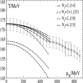
(a) (b)

Figure 2: (a) The transition line $T_{c}(\mu)$ for diferent number of flavors and masses in the range $m/T=0.1-0.4$, for the light quark mass. (b) The mass dependence of the transition line, for $N_{f}=3$ (Ref. 23).

In first order, the transition line for $N_{f}=2$ and $m/T=0.4$ is given by[10]

$$T_{c}(\mu_{q})/T_{c}(0)=1-0.070(35)\left(\mu_{q}/T_{c}(0)\right)^{2}.$$ (10)

As one can anticipate from Fig. 2(a), the mass dependence of $T_{c}(\mu)$ is rather small. Comparing $N_{f}=3$ results[23] (Fig. 2(b)) for $m/T=0.4$ and $m/T=0.02$ one finds however a significant mass dependents. As expected the curvature of the transition line becomes stronger with increasing mass. Using the perturbative asymptotic $\beta$-function in Eq. 9 gives

$$\frac{T_{c}(\mu_{q})}{T_{c}(0)}=\left\{\begin{array}[]{rl}1-0.025(6)\left(\frac{\mu_{q}}{T_{c}(0)}\right)^{2},&m/T=0.4\\ 1-0.114(46)\left(\frac{\mu_{q}}{T_{c}(0)}\right)^{2},&m/T=0.02\end{array}\right..$$ (11)

We note that an additional quark mass dependence is hidden here in the transition temperature at $\mu_{q}=0$, i.e. $T_{c}(0)$, which is used to normalize the transition temperature at $\mu_{q}\neq 0$. Furthermore, taking into account violations of asymptotic scaling in the $\beta$-function will lead to a further increase of the curvature of $T_{c}(\mu_{q})$.

This increase of the curvature can be understood as a result of much larger phase fluctuations for the smaller quark mass. A detailed analysis of the phase fluctuations can be found in Ref. Ejiri:2004yw. To make this more clear we have also calculated the transition line as a function of a vector chemical potential ($\mu_{V}\equiv\mu_{u}=-\mu_{d}$). This corresponds to reweighting with the absolute value of the determinant, i.e. the influence of the phase is dropped. In this case the mass dependence is much less significant:

$$\frac{T_{c}(\mu_{V})}{T_{c}(0)}=\left\{\begin{array}[]{rl}1-0.026(5)\left(\frac{\mu_{V}}{T_{c}(0)}\right)^{2},&m/T=0.4\\ 1-0.033(6)\left(\frac{\mu_{V}}{T_{c}(0)}\right)^{2},&m/T=0.02\end{array}\right..$$ (12)

Since for the larger quark mass the two transition lines are in good agreement, we have $T_{c}(\mu_{V})>T_{c}(\mu_{q})$ for $m/T=0.02$. This result seems to be a bit counter intuitive, since we know that the onset transition of isospin matter at $T=0$ takes place at $\mu_{V}=m_{\pi}/2$, rather than at $\mu_{q}=m_{B}/3$. However, this result can also be confirmed by the DOS method. In Fig. 3 we presents results[25] from a $4^{4}$ lattice and $N_{f}=4$.

(a) (b)

Figure 3: (a) The density of states $\rho$, the phase factor $\left<\cos\theta\right>$ and their product ²⁵. (b) Susceptibilites calculated for the DOS method, with and without the phase factor²⁵.

Simulations have been performed at finite isospin density with $\hat{\mu}_{V}=0.3$, according to Ref. Kogut:2002tm. The DOS ($\rho$) was defined according to Eq. 8 with $g=|\rm{det}M|\exp\{-S_{G}\}$ and $\phi=P$. In Fig. 3(a) we show $\rho$, the phase suppression factor $\left<cos(\theta)\right>$ and their product as a function of the constrained Plaquette $P$. We find, that the phase fluctuations in the low temperature phase ($P\raise 1.29167pt\hbox{$<$\kern-7.5pt\raise-4.73611pt\hbox{$\sim$}}2.8$) are much larger than in the high temperature phase ($P\raise 1.29167pt\hbox{$>$\kern-7.5pt\raise-4.73611pt\hbox{$\sim$}}2.8$). From this we can argue, that including the phase factor, the critical temperature will be lower than without the phase factor. Indeed, after calculating the susceptibilities from those distributions as a function of $\beta$, we find a shift in $\beta_{c}$ towards lower temperatures (see Fig. 3(b)). Moreover the value of $\beta_{c}$ is in good agreement with an earlier result form the reweighting method[8].

4 The critical end-point

The determination of the critical end-point on the transition line, separating a first order region form a crossover region is a difficult task. At present there are two different strategies used for this calculation. An infinite volume extrapolation of Lee-Yang Zeros[21, 22] and a finite size scaling analysis of susceptibilities and Binder Cumulants[27, 28, 13]. At this stage the most reliable calculation for the critical endpoint and physical quark masses comes form Ref. Fodor:2004nz. The result is $\mu_{B}=360(40)~{}\mbox{MeV}$ and $T=162(2)~{}\mbox{MeV}$. Note that those values are, however not yet free from corrections coming from the finite volume and lattice spacing.

In the case of 3 degenerate quarks the critical mass ($m_{c}(0)$), where the critical point sits at $\mu=0$, was determined. In this quantity huge cut-off effects were found. It was determined for standard staggered fermions[27] and $p4$ improved fermions[23], both on $N_{t}=4$ lattices. The outcomes for the critical pseudo scalar mass are $m_{\pi}^{\rm{crit}}=190(20)~{}\mbox{MeV},67(18)~{}\mbox{MeV}$, respectively. Binder Cumulant method also admits the determination of the universality class of this critical point, which was found to be that of a 3d-Ising model[27].

In addition the mass dependence of the critical point turned out to be rather large. A correct calculation of the critical point may thus only be possible, if the quark masses are known very precisely. The first Taylor coefficient of $m_{c}(\hat{\mu})$ was calculated in Ref. deForcrand:2003hx. The result of a combined fit for several lattice sizes and imaginary chemical potentials is

$$\frac{m_{c}(\mu)}{m_{c}(\mu=0)}=1+0.84(36)\left(\frac{\mu}{\pi T}\right)^{2},$$ (13)

where $m_{c}(\mu)$ is the critical quark mass. This coefficient does not look unnaturally small, since it was expanded in the natural units ($\mu/\pi T$), it will, however give in turn a rather large first coefficient for the critical chemical potential as a function of the quark mass ($\mu_{c}(m_{q})$).

Another interesting method to extract information about the critical end-point is the convergence radius of any bulk thermodynamic observable at $\mu=0$. As mentioned in Sec. 2.1, the Taylor expansion is limited by a phase transition. Thus for any $T<T_{\rm{endpoint}}\equiv T_{E}$ the convergence radius ($\rho$) should remain finite, whereas for $T>T_{E}$ it should be infinite. Since physical observables are even in $\hat{\mu}$, we have

$$\rho=\lim_{n\to\infty}\rho_{n}\equiv\lim_{n\to\infty}\sqrt{\left|c_{n}/c_{n+2}\right|}.$$ (14)

In Fig. 4(a) we show the absolute value of the Taylor coefficients of the pressure[6].

(a) (b)

Figure 4: (a) The absolute values of the Taylor coefficients of the pressure⁶. (b) The convergence radius of the pressure⁶.

The results are for $N_{f}=2$ and $m/T=0.4$. In Fig. 4(b) the first two terms in the series (Eq. 14) are drawn in a ($T,\mu$)-diagram, in order to compare with the phase transition line. As one can see in Fig. 4, for values of $T/T_{c}(0)\raise 1.29167pt\hbox{$>$\kern-7.5pt\raise-4.73611pt\hbox{$\sim$}}0.8$ the radius seems to increase. This corresponds to a critical chemical potential of $\mu_{E}\approx(3-3.6)T_{0}\approx(600-700)\mbox{MeV}$. This is a reasonably large value for $m_{q}/T=0.4$.

Note that the pressure and quark number density, which can be constructed from the coefficients in Fig. 4(a) is in good agreement with result from method 2.2 (Ref. Csikor:2004ik). Moreover the pressure is like the transition line, almost perfectly described by the leading order in $\mu/T$. For a further discussion of the pressure from Taylor expansion see Ref. ejiri.

5 Conclusions

For small $\mu/T$ several methods have been proposed and tested. The agreement between different methods is good. The phase diagram for small $\mu/T$ is slowly evolving and one can even address the question of locating the critical point. All methods are bases, however, on $\mu_{R}=0$ simulations and thus extrapolate. Moreover they give no solution for the sign problem and the results are not yet extrapolated to the continuum and infinite volume.

References

- [1] F. Karsch, E. Laermann and A. Peikert, Nucl. Phys. B605, 579 (2001).
- [2] S. Muroya et al., Prog. Theor. Phys. 110 615 (2003).
- [3] S. A. Gottlieb et al., Phys. Rev. D38, 2888 (1988).
- [4] S. Choe et al. [QCD-TARO Collaboration], Nucl. Phys. Proc. Suppl. 106, 462 (2002); Phys. Rev. D65, 054501 (2002); Nucl. Phys. A698, 395 (2002).
- [5] R. V. Gavai and S. Gupta, Phys. Rev. D68, 034506 (2003).
- [6] C. R. Allton et al., Phys. Rev. D68, 014507 (2003).
- [7] A. M. Ferrenberg and R. H. Swendsen, Phys. Rev. Lett. 61, 2635 (1988); Phys. Rev. Lett. 63 1195 (1989).
- [8] Z. Fodor and S. D. Katz, Phys. Lett. B534 87 (2002).
- [9] F. Csikor et al., JHEP 0405 046 (2004).
- [10] C. R. Allton et al., Phys. Rev. D66 074507 (2002).
- [11] P. de Forcrand et al., Nucl. Phys. Proc. Suppl. 119 541 (2003).
- [12] A. Roberge and N. Weiss, Nucl. Phys. B275 734 (1986).
- [13] P. de Forcrand and O. Philipsen, Nucl. Phys. B673 170 (2003);
- [14] P. de Forcrand and O. Philipsen, Nucl. Phys. B642 290 (2002).
- [15] M. D’Elia and M. P. Lombardo, Phys. Rev. D67 014505 (2003).
- [16] G. Bhanot et at., Phys. Lett. B187 381 (1987); Phys. Lett. B188 246 (1987); M.Karliner et al., Nucl. Phys. B302 204 (1988).
- [17] V. Azcoiti, G. di Carlo and A. F. Grillo, Phys. Rev. Lett. 65 2239 (1990).
- [18] X. Q. Luo, Mod. Phys. Lett. A16 1615 (2001).
- [19] A. Gocksch, Phys. Rev. Lett. 61 2054 (1988).
- [20] J. Ambjorn et al., JHEP 0210 062 (2002).
- [21] Z. Fodor and S. D. Katz, JHEP 0203 014 (2002).
- [22] Z. Fodor and S. D. Katz, JHEP 0404 050 (2004).
- [23] F. Karsch et al., Nucl. Phys. Proc. Suppl. 129 614 (2004).
- [24] S. Ejiri, Phys. Rev. D69 094506 (2004).
- [25] Z. Fodor, S. Katz and C. Schmidt, in preparation.
- [26] J. B. Kogut and D. K. Sinclair, Phys. Rev. D66 014508 (2002); Phys. Rev. D66 034505 (2002).
- [27] F. Karsch, E. Laermann and C. Schmidt, Phys. Lett. B520 41 (2001).
- [28] N. H. Christ and X. Liao, Nucl. Phys. Proc. Suppl. 119 514 (2003).
- [29] S. Ejiri, this proceedings.