DFTT 18/04

SISSA 59/2004/FM

IFUM-793-FT

Amplitude ratios for the mass spectrum of the 2d Ising model in the high-$T,~{}H\neq 0$ phase

M. Caselle^a, P. Grinza^b and A. Rago^c

^a Dipartimento di Fisica Teorica dell’Università di Torino and I.N.F.N.,

via P.Giuria 1, I-10125 Torino, Italy

^b SISSA and I.N.F.N, via Beirut 2-4, I-34014 Trieste, Italy

^c Dipartimento di Fisica Teorica dell’Università di Milano and I.N.F.N.,

Via Celoria 16, I-20133 Milano, Italy

We study the behaviour of the 2d Ising model in the symmetric high temperature phase in presence of a small magnetic perturbation. We successfully compare the quantum field theory predictions for the shift in the mass spectrum of the theory with a set of high precision transfer matrix results. Our results rule out a prediction for the same quantity obtained some years ago with strong coupling methods.

1 Introduction.

Despite its apparent simplicity and the fact that since 1944 the exact expression of the free energy along the $h=0$ axis is known exactly [1] the two dimensional Ising model is still an endless source of interesting and challenging problems [2]-[24].

In particular in these last few years a renewed interest has been attracted by the study of the model in its whole complexity, i.e. in presence of both magnetic and thermal perturbations. There are two main reasons behind this renewed interest. On one side recent progress in 2d quantum field theory (in particular, but not only, in the framework of perturbed CFT’s and S-matrix integrable models) allowed to obtain a host of new important results on correlation functions, amplitude ratios and more generally on perturbations around integrable directions [2]-[15]. On the other side the appearance of new powerful algorithms (both for montecarlo simulations and for transfer matrix studies) and the increasing performances of computers allowed to precisely test a lot of the above predictions [16]-[24]. This paper, which is devoted to the study of Ising model in presence of a small magnetic perturbation around the integrable thermal axis, is a further step in this direction. It can be considered as the natural continuation of [16] in which, with similar tools, the opposite setting of a small thermal perturbation around the magnetic integrable line was studied and it is part of our more general ongoing project [13]-[24] on the study and characterization of the 2d Ising model in the whole thermal and magnetic plane. A further reason of interest for the present analysis is the theoretical estimate recently obtained by Fonseca and Zamolodchikov [4] for the first order magnetic correction to the mass spectrum of the model. This estimate turns out to be in sharp disagreement (more than one order of magnitude) with a previous estimate of the same constant obtained more than 20 years ago with strong coupling methods in [25]. This disagreement is very puzzling, since strong coupling estimates in the 2d Ising model are usually highly reliable. One of the goals of the present work is to fix this disagreement testing these two estimates with a high precision transfer matrix calculation directly in the 2d Ising model. This paper is organized as follows. In sect. 2 we first recall some known results on the 2d Ising model and then concentrate on the definitions and theoretical predictions for the quantities which we measure in our transfer matrix analysis. Sect. 3 is devoted to a short discussion of the transfer matrix method while in the last section we discuss our results and compare our findings with the theoretical predictions.

2 The model.

In this section we briefly recall some well known results on the Ising model. A more detailed description can be found in the reviews[26]-[29].

2.1 The lattice version of the model.

The Ising model in a magnetic field is defined by the partition function

$$Z=\sum_{\sigma_{i}=\pm 1}e^{\beta(\sum_{\langle n,m\rangle}\sigma_{n}\sigma_{m}+H\sum_{n}\sigma_{n})}$$ (1)

where the field variable $\sigma_{n}$ takes the values $\{\pm 1\}$; $n\equiv(n_{0},n_{1})$ labels the sites of a square lattice size $L_{0}$ and $L_{1}$ in the two directions and lattice spacing $a$. $\langle n,m\rangle$ denotes nearest neighbor sites on the lattice. In the following we shall treat asymmetrically the two directions. We shall denote $n_{0}$ as the compactified “time” coordinate and $n_{1}$ as the space one. The number of sites of the lattice will be denoted by $N\equiv L_{0}L_{1}$. The lattice extent in the transverse (“time”) direction will be denoted as $L_{0}$. Following the standard notation we define $h_{l}=\beta H$ thus the partition function becomes:

$$Z(h_{l})=\sum_{\sigma_{i}=\pm 1}e^{\beta\sum_{\langle n,m\rangle}\sigma_{m}\sigma_{m}+h_{l}\sum_{n}\sigma_{n}}\;\;\;.$$ (2)

As it is well known the 2d Ising model has a second order phase transition at $h_{l}=0$ and $\beta=\beta_{c}$ given by:

$$\beta=\beta_{c}=\frac{1}{2}\log{(\sqrt{2}+1)}=0.4406868...$$

In the following we shall be interested in the high temperature phase of the model (i.e. $\beta<\beta_{c}$) in which the $\mathbb{Z}_{2}$ symmetry is unbroken.

2.2 Continuum theory

In the continuum limit the model is described by the action:

$${\cal A}={\cal A}_{0}-\tau\int d^{2}x\,\varepsilon(x)-h\int d^{2}x\,\sigma(x)\,,$$ (3)

where $\sigma(x)$ and $\varepsilon(x)$ denote the magnetic and thermal perturbing operators respectively while $h$ and $\tau$ are dimensional couplings measuring the magnetic field and the deviation from critical temperature. A standard scaling analysis shows that the scaling behaviour of these two couplings is

$$\tau\sim m^{2-x_{\varepsilon}}=m\,,$$

$$h\sim m^{2-x_{\sigma}}=m^{15/8}$$ (4)

where $m\sim 1/\xi$ ($\xi$ being the correlation length of the model) denotes the mass scale associated to the breaking of scale invariance away from criticality, $x_{\varepsilon}=1$ and $x_{\sigma}=1/8$ are the scaling dimensions of the energy and spin operators respectively and ${\cal A}_{0}$ denotes the conformal invariant action at the critical point. In the Ising case, which is known to be described by a free massless Majorana fermion, this can be written explicitly as:

$${\cal A}_{0}=\frac{1}{2}\int d^{2}x\,(\psi\bar{\partial}\psi+\bar{\psi}\partial\bar{\psi})\,,$$ (5)

where $\partial=\partial_{z}=(\partial_{1}-i\partial_{2})/2$ and $\bar{\partial}=\partial_{\bar{z}}=(\partial_{1}+i\partial_{2})/2$ and the operators $\psi$ and $\bar{\psi}$ are the two components of the neutral Majorana fermion.

The thermal perturbing operator (which coincides with the energy operator) can be written as

$$\varepsilon\sim\bar{\psi}\psi\,;$$ (6)

which allows to identify it as the mass term of the free fermionic action, in agreement with the first of the scaling equations (4).

By combining the two scaling equations (4) one can see that the field theory (3) describes a one-parameter family of renormalization group trajectories flowing out of the critical point at $\tau=h=0$ and labeled by the dimensionless quantity

$$\eta=\frac{\tau}{|h|^{8/15}}\,\,.$$ (7)

The Ising field theory can be solved exactly in the two limiting cases of $h=0$ and $\tau=0$. In the first case, as we have seen above, it is simply the theory of free massive fermion, the mass being proportional to $|\tau|$. In the second case (which corresponds in the lattice discretization to the magnetic perturbation with $\beta$ fixed to the critical value $\beta=\beta_{c}$) A. Zamolodchikov was able to show that (3) with $\tau=0$ is a complicated but integrable quantum field theory [2] of eight interacting particles.

For generic values of $h$ and $\tau$ exact integrability is lost but notwithstanding this some important theoretical results can all the same be obtained. Let us see a few of them.

• Equation of state.

  With a combination of transfer matrix techniques and analytic continuation of suitable parametric representations it is possible to construct a very precise expansion for Helmholtz free energy of the the model and from it of the equation of state in the whole critical region in the $(\tau,h)$ plane [21]. From this expression precise predictions for several universal amplitude ratios can be obtained (see [21] for details).

• The spectrum of the model. This important result was conjectured for the first time in a seminal paper of Mc Coy and Wu [30] and recently re–understood in a field theoretic language (see [29] for a thorough discussion). The scenario which emerges is the following. For $\eta=-\infty$ (i.e. in the low temperature broken symmetry phase) the spectrum starts with a cut. In this limit the natural degrees of freedom of the model are kinks interpolating between the two degenerate vacua which are non-local with respect to the spin degrees of freedom of the model. As the magnetic field is switched on (i.e. for large and negative values of $\eta$) this cut breaks up in a host of particles which may be understood as bound states of the above mentioned kinks. As $\eta$ is increased from $-\infty$ to finite negative values the number of stable particles (i.e. below the pair creation threshold $m_{n}<2m_{1}$) decreases. Exactly at $\eta=0$ only three such particles are left (but, only for this value of $\eta$, due to the exact integrability of the model five more particles turn out to be stable even if they are above threshold). The number of stable particles continues to decrease as $\eta$ increases, until a single particle is left at large enough $\eta$. There is a wide region of values of $\eta$ before the positive thermal axis (i.e. $\eta=+\infty$) is reached in which the spectrum contains only one stable particle. This is the region in which we shall perform our analysis in the following.

  

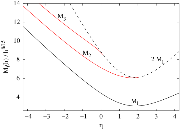
  Figure 1: Ising Model’s masses, the value of the masses has been obtained in [3]

• Small perturbations around the integrable lines. The most interesting result for our present purposes is that in the nearby of the two integrable lines a few exact results can be obtained using perturbative methods. In particular one can evaluate the corrections to the masses and to the ground state energy due to the perturbing operator [7]. Again we have two possible situations:

  a] A small thermal perturbation of the Zamolodchikov’s integrable model along the $\tau=0$ magnetic axis. Estimates for the first order mass correction where obtained in [7] and successfully tested both on the lattice, using transfer matrix methods [16] and directly in the Ising field theory by a numerical diagonalization of the Hamiltonian on a conformal basis of states [7].

  b] A small magnetic perturbation of the free fermionic theory along the $h=0$ axis. This case was recently studied by Fonseca and Zamolodchikov [4] which were able to obtain, using the Ward identities of the model, the matrix elements of the product $\sigma(x)\sigma(x^{\prime})$ between any particle states. This is exactly the ingredient which is needed to obtain the sought for mass correction. The aim of our paper is to test this result with a transfer matrix analysis directly on the lattice model. We shall devote the next subsection to a detailed discussion of this term.

2.3 The mass correction

Following the above discussion in the $\tau>0$ phase, for small value of $h$ there is a single stable particle in the spectrum. Let us call $m(\tau,h)$ its mass. For symmetry reasons the correction to the mass of the particle when the magnetic field is switched on at $\tau>0$ must be proportional to $h^{2}$. Scaling arguments (see the discussion in the previous section) then fix the dependence on $\tau$ to be $\tau^{-15/4}$. Thus we expect the following behaviour:

$$m(\tau,h)=m(\tau,0)(1+\hat{a}h^{2}\tau^{-15/4})$$ (8)

From a numerical point of view it is useful to rewrite this dependence as a function of the unperturbed mass $m(\tau,0)$:

$$m(\tau,h)=m(\tau,0)(1+ah^{2}m(\tau,0)^{-15/4})$$ (9)

Recently, in a remarkable paper Fonseca and Zamolodchikov [4] were able to evaluate analytically this constant which turns out to be

$$a=10.7619899(1)$$ (10)

The above correction can also be rewritten in a form which will be useful in the following:

$$m^{2}(\tau,h)=m^{2}(\tau,0)+\tilde{a}h^{2}\tau^{-7/4}$$ (11)

These three constants, which are actually the same constant written in different units, can be easily related among them. In fact, thanks to the fact that the Ising quantum field theory is solved exactly along the thermal line, the relation between $\tau$ and $m(\tau,0)$ is know exactly: $m=2\pi\tau$. This allows to write the following relations:

$$\tilde{a} = 2a(2\pi)^{-7/4}$$ (12)

$$\hat{a} = a(2\pi)^{-15/4}$$ (13)

2.3.1 Theoretical estimates for mass correction

Up to a few months ago the only existing estimate for the constant $a$ was the one reported in [25], obtained performing the continuum limit extrapolation of the strong coupling expansion of the perturbed two point correlator :

$$a=(\frac{1}{4}+\frac{1}{\pi})(2\sqrt{2})^{\frac{1}{4}}=0.73700676...$$ (14)

This estimate was never tested with numerical simulations or transfer matrix methods. Further, the impressive discrepancy between (10) and the above estimate was one of the major reasons which prompted us to perform the present transfer matrix analysis.

2.4 Correction in the free energy.

Similarly to the mass case one can define the deviation from the unperturbed value of the free energy ${\cal F}$ (which is nothing else than the lowest eigenvalue of the transfer matrix spectrum). In this case it is easy to obtain a theoretical estimate of this deviation by noticing that for symmetry reasons the first nonzero correction must be again at order $h^{2}$ and is exactly given by $1/2$ times the magnetic susceptibility

$${\cal F}(\tau,h)={\cal F}(\tau,0)+\frac{h^{2}}{2}\chi_{+}(\tau,0)+{\cal O}(h^{4})\equiv{\cal F}(\tau,0)+\frac{\Gamma_{+}}{2}h^{2}\tau^{-7/4}+...$$ (15)

Where in the last term of the above equation $\Gamma_{+}$ denotes the susceptibility amplitude and we have inserted the known dependence on $\tau$ of the susceptibility. An important role in the following analysis is played by the fact that the value of $\Gamma_{+}$ in the the continuum theory is known exactly (see for instance [29]):

$$\Gamma_{+}=0.148001214...\,.$$ (16)

2.5 Universal amplitude ratios.

A major problem in comparing the above values, obtained in the continuum limit QFT, with our numerical estimates in the lattice model is that we must convert the continuum limit parameters $\tau$ and $h$ into their lattice counterparts $t$ and $h_{l}$. A nice way to avoid this problem is to combine the above constants in a suitable universal ratio which is thus independent from the particular realization of the underlying quantum field theory. There are two natural choices:

• Following [29] we shall study the combination

  $$R_{1}=\lim_{\eta\to\infty}\frac{\delta m^{2}}{\delta{\cal F}}$$ (17)

  where

  $$\delta m^{2}\equiv m^{2}(\tau,h)-m^{2}(\tau,0)$$ (18)

  $$\delta{\cal F}\equiv{\cal F}(\tau,h)-{\cal F}(\tau,0)$$ (19)

  A direct substitution gives:

  $$\lim_{\eta\to\infty}\frac{\delta m_{1}^{2}}{\delta{\cal F}}=\frac{4a}{\Gamma_{+}(2\pi)^{7/2}}$$ (20)

• A second option is:

  $$R_{2}=\frac{\delta m}{m(\tau,0)}\frac{M_{s}^{2}(-\tau)}{M^{2}(\tau,h)}$$ (21)

  where

  $$\delta m\equiv m(\tau,h)-m(\tau,0)$$ (22)

  while $M(\tau,h)$ denotes the magnetization and $M_{s}(-\tau)$ the spontaneous magnetization. A direct substitution of the various terms leads to

  $$R_{2}=a(2\pi)^{-15/4}\frac{B^{2}}{\Gamma^{2}_{+}}$$ (23)

  where $B$ denotes the amplitude of the spontaneous magnetization whose value is known exactly in the continuum limit theory (see for instance [29])

  $$B=1.70852190.$$ (24)

The expected values for these ratios, using the Fonseca-Zamolodchikov estimate for the constant $a$ are

$$R_{1}=11.66467...\hskip 56.9055ptR_{2}=1.4568962...$$ (25)

while with the strong coupling estimate for $a$ we should expect:

$$R_{1}=0.7988246...\hskip 56.9055ptR_{2}=0.09977173...$$ (26)

2.6 Lattice amplitudes.

This is all we can do for a generic realization of the Ising quantum field theory. However in the particular case of the 2d square lattice realization thanks to the fact that the model is exactly solved also on the lattice for $h=0$ we know the value of several of the above amplitudes directly in the lattice realization. The mass of the theory in the transfer matrix geometry is

$$m_{\ell}=-\log~{}v\left(\frac{1+v}{1-v}\right)$$ (27)

with $v=\tanh\beta$. The index $\ell$ recalls that this is the lattice estimate of the mass of the model. Eq.(27) leads to the following expansion in the vicinity of the critical point

$$m_{\ell}(t,0)\sim 4\beta_{c}t$$ (28)

where $t$ is the reduced temperature defined as

$$t=\frac{|\beta-\beta_{c}|}{\beta_{c}}.$$ (29)

The spontaneous magnetization is given by

$$M_{s}=\left(1-\frac{1}{sh^{4}(2\beta)}\right)^{\frac{1}{8}}$$ (30)

which gives:

$$M_{s}\sim(-8\sqrt{2}\beta_{c}~{}t)^{\frac{1}{8}}.$$ (31)

For the magnetic susceptibility $\chi_{+}(t)$ there is no exact expression. However this observable has been studied extensively in the past years, firstly by McCoy et al. [31] and more recently by Orrick et al. [32] using strong coupling expansions (notice that the first term in the expansion in powers of $t$ can be evaluated exactly). One finds:

$$\chi_{+}(t)=C_{0,+}t^{-7/4}+C_{1,+}t^{-3/4}+\dots$$ (32)

where

$$C_{0,+} = 0.962581732\dots$$

$$C_{1,+} = 0.074988153\dots\;.$$ (33)

Plugging these amplitudes (together with the lattice estimate of the constant $a$ which we shall discuss in the following section) it is possible to obtain the two ratios $R_{1}$ and $R_{2}$ discussed in the previous section.

Another possible use of these results is to construct the explicit relation between $t$ and $\tau$ and similarly between $h_{\ell}$ and $h$. This will allow us to test separately the two predictions eq.(8) and (15). Comparing the lattice and continuum values for the mass we find:

$$\tau=\frac{\log(1+\sqrt{2})}{\pi}t\equiv k_{\tau}\;t,\ \ \ \$$ (34)

while comparing the susceptibility amplitudes

$$C_{0,+}=k_{\tau}^{-7/4}k_{h}^{2}\;\Gamma_{+}$$ (35)

we find

$$h=2^{5/48}e^{1/8}A^{-3/2}h_{l}\equiv k_{h}\;h_{\ell}$$ (36)

(where $A=1.28242712\dots$ is the Glaisher constant).

With these results at hand we may write an explicit prediction for the constant $a$ directly on the lattice. Defining the lattice version of $a$ as:

$$a_{\ell}\equiv k_{h}^{2}k_{\tau}^{-15/4}~{}a$$ (37)

we find using the value for $a$ obtained by Fonseca and Zamolodchikov [4]

$$a_{\ell}=7.56977\dots$$ (38)

and, using the strong coupling one discussed in [25]:

$$a_{\ell}=0.518396\dots\,.$$ (39)

In the following we shall use this last result and shall directly extract from the transfer matrix data the value of $a_{\ell}$ which we shall then combine with the other amplitudes in order to obtain the two universal ratios $R_{1}$ and $R_{2}$.

3 The transfer matrix analysis

For the analysis of the transfer matrix data we followed the same procedure of our previous works [16, 17, 24] which can be schematically sketched as follow.

• We evaluate the first few eigenvalues of the transfer matrix for the values of temperature and magnetic coupling in which we are interested for lattice widths in the transverse direction in the range $L\in\{9-21\}$. We construct from them the observables in which we are intested (mass and free energy) and extrapolate their infinite lattice limits using the recursive procedure discussed in detail the appendix of [22].

• For each values of $t$ and $h_{\ell}$ we construct the combinations $\delta m$ and $\delta m^{2}$ and $\delta{\cal F}$ defined in eq.(22), (18) and (19):

• We fit $\delta m^{2}$, $\delta m$ and $\delta{\cal F}$ assuming the known scaling behaviour for these quantities. As we shall see the first few terms of the scaling functions will be enough to obtain stable results for the fits within the precision of our data.

In table (1) we report the parameters and the various settings we used in our simulations, while in tables (2,3) we report a sample of our data to allow the interested reader to reproduce our analysis.

$t$	$h_{\ell}$	$L$
0.345	0.0	9
0.350	0.0003	10
0.355	0.0005	11
0.360	0.0008	$\vdots$
0.365	0.0010
0.370	0.0013
	0.0015	19
	0.0018	20
	0.0020	21

Table 1: Parameters value.

$L$	$1/m(t,h_{\ell})$	${\mathcal{F}(t,h_{\ell})}$	$M_{\ell}(t,h_{\ell})$
15	2.565917754587	0.830031898983	0.020167928578
16	2.565918168084	0.830031896272	0.020167777385
17	2.5659182662035	0.830031895299	0.020167731420
18	2.565918247605	0.830031894746	0.020167716025
19	2.565918227627	0.830031894142	0.020167710600
20	2.565918215050	0.830031894612	0.020167708951
21	2.565918209646	0.830031893614	0.020167708217
$\infty$	2.56591821(1)	0.830031894(1)	0.020167708(1)

Table 2: Example of data used for the extrapolation ($h_{\ell}=0.0013$, $\beta=0.350$).

4 Discussion of our results.

Now we are in the position to compare the lattice results, coming from the transfer matrix approach, with the field theoretic estimates of the ratios $R_{1}$, $R_{2}$. To this aim, the first step is to extract the leading behaviour of $\delta m$, $\delta m^{2}$, $\delta{\mathcal{F}}$ and $M_{\ell}(t,h_{\ell})$ from the data obtained by means of the transfer matrix.

As a preliminary check of our procedure we estimated from the transfer matrix data the mass at zero magnetic field which in this geometry is known exactly and is given by eq.(27). We report in tab.4 the comparison which turns out to be fully satisfactory.

Then we concentrated in the evaluation of $\delta m^{2}$. Symmetry considerations suggest the following expansion in even powers of $h_{\ell}$ for this quantity.

$$\delta m^{2}=f_{1}(t)h_{\ell}^{2}+f_{2}(t)h_{\ell}^{4}+\dots$$ (40)

It turns out that, within the precision of our data and given our choice of values of $h_{\ell}$, it is enough to take into account only the first two terms in this fit, the term proportional to $h^{6}$ being completely negligible. For each fixed value of $t$ we extract from the fit the best fit values for $f_{1}(t)$ and $f_{2}(t)$. Since we are interested in the leading behaviour of $\delta m^{2}$, in the following we shall concentrate in the study of the function $f_{1}(t)$. The functional form of $f_{1}(t)$ can be easily constructed using the same RG and CFT arguments developed in [20]-[22], [16]:

$$f_{1}(t)=\tilde{a}_{\ell}t^{-7/4}+a_{1}t^{-3/4}+a_{2}t^{1/4}+\dots$$ (41)

where $\tilde{a}_{\ell}$ is the amplitude in which we are interested.
Following the same fitting procedure used in [16], we obtain:

$$\tilde{a}_{\ell}=5.61\pm 0.01$$ (42)

which gives

$$a_{\ell}=7.56\pm 0.01$$ (43)

in complete agreement with the Fonseca-Zamolodchikov estimate of the amplitude $a$ (see eq. (38)).

$h_{\ell}$	$\beta=0.345$	$\beta=0.350$	$\beta=0.355$	$\beta=0.360$
0	2.42236580(1)	2.56721580(1)	2.72886532(1)	2.91043999(6)
0.0003	2.42231285(1)	2.56714664(1)	2.72877368(1)	2.91031661(4)
0.0005	2.42221873(1)	2.56702370(1)	2.72861080(1)	2.91009730(5)
0.0008	2.42198936(1)	2.56672412(1)	2.72821391(1)	2.90956300(5)
0.0010	2.42177770(1)	2.56644770(1)	2.72784773(1)	2.90907012(4)
0.0013	2.42137222(1.5)	2.56591821(1)	2.72714641(1)	2.90812629(4)
0.0015	2.42104331(1)	2.56548878(1)	2.72657770(2)	2.90736112(3)
0.0018	2.42046226(1)	2.56473025(1)	2.72557340(1)	2.90601025(2)
0.0020	2.42001655(1)	2.56414851(1)	2.72480337(1)	2.90497486(3)
(a) Inverse mass $1/m(t,h_{\ell})$

$h_{\ell}$	$\beta=0.345$	$\beta=0.350$	$\beta=0.355$	$\beta=0.360$
0.	0.825668076(1)	0.830018782(1)	0.8344669273(3)	0.839014965(1)
0.0003	0.825668712(1)	0.830019481(1)	0.834467698(1)	0.839015821(1)
0.0005	0.825669843(1)	0.830020722(1)	0.834469068(1)	0.839017342(1)
0.0008	0.825672600(1)	0.830023748(1)	0.834472408(1)	0.839021049(1)
0.0010	0.825675145(1)	0.830026541(1)	0.834475490(1)	0.839024471(1)
0.0013	0.825680021(1)	0.830031894(1)	0.834481397(1)	0.839031028(1)
0.0015	0.825683978(1)	0.830036238(1)	0.834486189(1)	0.839036348(1)
0.0018	0.825690973(1)	0.830043915(1)	0.834494660(1)	0.839045750(1)
0.0020	0.825696341(1)	0.830049807(1)	0.834501162(1)	0.839052965(1)
(b) Free energy ${\mathcal{F}}(t,h_{\ell})$

$h_{\ell}$	$\beta=0.345$	$\beta=0.350$	$\beta=0.355$	$\beta=0.360$
0.0003	0.004241449(1)	0.004655977(1)	0.005138273(1)	0.00570442(1)
0.0005	0.007068848(1)	0.00775956(1)	0.00856335(1)	0.00950676(1)
0.0008	0.011309247(1)	0.012414204(1)	0.01369968(1)	0.01520845(1)
0.0010	0.014135509(1)	0.015516337(1)	0.017122651(1)	0.019007841(5)
0.0013	0.018373549(1)	0.020167708(1)	0.022254596(1)	0.024703401(2)
0.0015	0.021197803(1)	0.023267128(1)	0.0256738415(5)	0.028497574(2)
0.0018	0.025432177(1)	0.027913548(1)	0.030798990(1)	0.034183633(2)
0.0020	0.028253554(1)	0.031009083(1)	0.034212903(1)	0.037970351(1)
(c) Magnetization $M(t,h_{\ell})$

Table 3: Extrapolated values of different operators as function of the magnetic coupling and the temperature.

$\beta$	Exact mass formula	Transfer matrix
$0.345$	$2.4223658021832$	$2.42236580(1)$
$0.350$	$2.5672157958004$	$2.56721580(1)$
$0.355$	$2.7288653104825$	$2.72886532(1)$
$0.360$	$2.9104399518676$	$2.91043999(5)$
$0.365$	$3.1158911582069$	$3.115891(1)$
$0.370$	$3.3502882801313$	$3.350287(1)$

Table 4: Comparison of our TM extrapolation with the exact result for the invers mass at zero magnetic field

The amplitude of the leading behaviour of $\delta m$ can be immediately inferred from that of $\delta m^{2}$

$$\delta m = \frac{\tilde{a}_{\ell}}{2m_{\ell}(t,0)}t^{-7/4}h_{\ell}^{2}+\dots$$

$$= \frac{\tilde{a}_{\ell}}{8\beta_{c}}t^{-11/4}h_{\ell}^{2}+\dots$$

$$\equiv \tilde{b}_{\ell}\,t^{-11/4}h_{\ell}^{2}+\dots$$ (45)

plugging in the last definition the above obtained value of $\tilde{a}_{\ell}$ we obtain

$$\tilde{b}_{\ell}=1.591\pm 0.002.$$ (46)

As a consistency check, we computed the same amplitude directly from the fit of the transfer matrix data. The final result is

$$\tilde{b}_{\ell}=1.592\pm 0.003$$ (47)

which is completely equivalent to the previous estimate.

To estimate the vacuum energy on the lattice let us notice first of all that $\delta{\mathcal{F}}$ can be expanded as

$$\delta{\mathcal{F}}=\frac{1}{2}\chi_{+}(t)h_{\ell}^{2}+g_{2}(t)h_{\ell}^{4}+\dots$$ (48)

where the function $\chi_{+}(t)$ is the magnetic susceptibility of the model in the high-temperature phase $\beta<\beta_{c}$ and $h=0$ already discussed in section 2.6. Hence the exact estimate of the amplitude $\tilde{c}_{\ell}$ of the free energy on the lattice is given by

$$\tilde{c}_{\ell}=\frac{C_{0,+}}{2}=0.48129086\dots\;.$$ (49)

We also compared the previous exact results (quoted in sect. 2.6) with our numerical estimates. We found

$$C_{0,+}^{\textrm{\tiny num}} = 0.962\pm 0.002$$

$$C_{1,+}^{\textrm{\tiny num}} = 0.075\pm 0.001$$

in complete agreement with (33).

Finally, we need the amplitude $\tilde{d}_{\ell}$ of the scaling behaviour of the magnetization. It can be easily computed (exactly) from the definition of $M_{\ell}(t,h_{\ell})$

$$M_{\ell}(t,h_{\ell})=\frac{\partial\mathcal{F}}{\partial h_{\ell}}=C_{0,+}\,t^{-7/4}h+\dots$$ (50)

leading to

$$\tilde{d}_{\ell}=C_{0,+}=0.962581732\dots\,.$$ (51)

Since the transfer matrix approach allows also the numerical computation of the magnetization, we can extract the numerical estimate of $\tilde{d}_{\ell}$

$$\tilde{d}_{\ell}=0.961\pm 0.004$$ (52)

which, once again, agrees with the previous results. We also stress that the zero-field quantities $m_{\ell}$ and $M_{s}$ involved in the ratio $R_{2}$ are given by their exact expressions quoted in section 2.6.

The final step is then to compute the lattice estimates of the ratios $R_{1}$, $R_{2}$

$$R_{1} = \frac{\tilde{a}_{\ell}}{\tilde{c}_{\ell}}=11.66\pm 0.02$$

$$R_{2} = 2^{-9/8}\beta_{c}^{-3/4}\frac{\tilde{b}_{\ell}}{\tilde{d}_{\ell}^{2}}=1.456\pm 0.002$$ (53)

which agree with the field theoretic predictions obtained using the Fonseca and Zamolodchikov estimate of the constant $a$ (see eq. (25)).

The precision of our numerical computations allows to rule out unambiguosly the strong coupling estimates of these universal ratios.

It would be interesting to investigate the reasons of this failure, which is even more surprising given the usual high reliability of strong coupling results in two dimensional statistical models (and in particular in the Ising model). A possible explanation is that the result of [25] is based on a peculiar mutipole expansion of the perturbed two point function, which was proved to have good converegence properties when tested in the case of the $H=0$ susceptibility (see [31]) but most probably has a less good behaviour if one is interested in the mass shift.

Acknowledgments. We would like to thank G. Delfino for useful discussions. This work was partially supported by the European Commission TMR programme HPRN-CT-2002-00325 (EUCLID). The work of P.G. is supported by the COFIN “Teoria dei Campi, Meccanica Statistica e Sistemi Elettronici”.

References

- [1] L. Onsager, Phys. Rev. 65 (1944) 117.
- [2] A. B. Zamolodchikov, Adv. Stud. Pure Math. 19 (1989) 641, A. B. Zamolodchikov, Int. J. Mod. Phys. A 4 (1989) 4235.
- [3] P. Fonseca and A. Zamolodchikov, J. Stat. Phys. 110 (2003) 527, [arXiv:hep-th/0112167].
- [4] P. Fonseca and A. Zamolodchikov, [arXiv:hep-th/0309228].
- [5] V. A. Fateev, Phys. Lett. B 324 (1994) 45.
- [6] V. Fateev, S. Lukyanov, A. B. Zamolodchikov and A. B. Zamolodchikov, Nucl. Phys. B 516 (1998) 652. [arXiv:hep-th/9709034].
- [7] G. Delfino, G. Mussardo and P. Simonetti, Nucl. Phys. B 473 (1996) 469 [arXiv:hep-th/9603011].
- [8] G. Delfino and G. Mussardo, Nucl. Phys. B 455 (1995) 724. [arXiv:hep-th/9507010].
- [9] G. Delfino, Phys. Lett. B 419 (1998) 291 [Erratum-ibid. B 518 (1998) 330]. [arXiv:hep-th/9710019].
- [10] G. Delfino, J. Phys. A 34 (2001) L161. [arXiv:hep-th/0101180].
- [11] A. Leclair and G. Mussardo, Nucl. Phys. B 552 (1999) 624. [arXiv:hep-th/9902075].
- [12] G. Mussardo, J. Phys. A 34, 7399 (2001). [arXiv:hep-th/0103214].
- [13] P. Grinza and N. Magnoli, J. Phys. A 36 (2003) L509 [arXiv:hep-th/0306100].
- [14] P. Calabrese, M. Caselle, A. Celi, A. Pelissetto and E. Vicari, J. Phys. A 33 (2000) 8155 [arXiv:hep-th/0005254].
- [15] M. Caselle, P. Grinza, R. Guida and N. Magnoli, J. Phys. A 37 (2004) L47 [arXiv:hep-th/0306086].
- [16] P. Grinza and A. Rago, Nucl. Phys. B 651 (2003) 387 [arXiv:hep-th/0208016].
- [17] M. Caselle and M. Hasenbusch, Nucl. Phys. B 579 (2000) 667. [arXiv:hep-th/9911216].
- [18] M. Caselle, P. Grinza and N. Magnoli, Nucl. Phys. B 579 (2000) 635. [arXiv:hep-th/9909065].
- [19] M. Caselle, P. Grinza and N. Magnoli, J. Phys. A 34 (2001) 8733. [arXiv:hep-th/0103263].
- [20] M. Caselle, M. Hasenbusch, A. Pelissetto and E. Vicari, J. Phys. A 35 (2002) 4861 [arXiv:cond-mat/0106372].
- [21] M. Caselle, M. Hasenbusch, A. Pelissetto and E. Vicari, J. Phys. A 34 (2001) 2923 [arXiv:cond-mat/0011305].
- [22] M. Caselle, M. Hasenbusch, A. Pelissetto and E. Vicari, J. Phys. A 33 (2000) 8171 [arXiv:hep-th/0003049].
- [23] M. Caselle and M. Hasenbusch, Nucl. Phys. B 639 (2002) 549 [arXiv:hep-th/0204088].
- [24] P. Grinza and A. Rago, J. Phys. A 37 (2004) L4701, [arXiv:cond-mat/0210046].
- [25] S. S. Salihoglu, Phys. Rev. D 24 (1981) 3255.
- [26] B. M. McCoy and T. T. Wu, The two dimensional Ising Model, (Harvard Univ. Press, Cambridge,1973);
- [27] B. M. McCoy, in Statistical Mechanics and Field Theory, eds. V.V. Bazhanov and C.J. Burden, (World Scientific, Singapore, 1995).
- [28] G. Delfino, Phys. Lett. B 419 (1998) 291 [Erratum-ibid. B 518 (2001) 330] [arXiv:hep-th/9710019].
- [29] G. Delfino, J. Phys. A 37 (2004) R45, [arXiv:hep-th/0312119].
- [30] B.M. McCoy and T.T. Wu, Phys. Rev. D 18 (1978) 1259.
- [31] T. T. Wu, B. M. McCoy, C. A. Tracy and E. Barouch, Phys. Rev. B 13 (1976) 316.
- [32] W. P. Orrick, B. Nickel, A. J. Guttmann, J. H. H. Perk, J. Statist. Phys. 102 (2001) 795-841; and W. P. Orrick, B. G. Nickel, A. J. Guttmann, J. H. H. Perk Phys. Rev. Lett. 86 (2001) 4120-4123.