Cold, dense matter via the lattice NJL model

Abstract

We simulate the lattice Nambu–Jona-Lasinio (NJL) model in $3+1$-dimensions at non-zero baryon chemical potential ($\mu$) and zero temperature ($T$) and treat the results as phenomenologically relevant for cold, dense quark matter. Measurements of the chiral condensate indicate a crossover in the thermodynamic limit, whilst at high chemical potential and zero temperature we observe a non-zero diquark condensate and a gap in the fermion dispersion relation, which together provide evidence for BCS superfluidity. In particular, the size of gap is found to be approximately $15\%$ the value of the vacuum fermion mass and roughly independent of $\mu$ in the chirally restored phase.

I Introduction

Whilst many of the talks at this workshop have been concerned with QCD at extreme temperatures, the “extreme environment” in the work presented here is that of cold, dense matter, where QCD is believed to exhibit colour superconductivity via the condensation of diquarks analogous to the Cooper pairs of BCS superconductors (for recent reviews on colour superconductivity see e.g. Rajagopal and Wilczek (2001); Rischke (2004)). The BCS mechanism in a superconductor is a subtle one, since the fundamental interaction between electrons is repulsive and the net attractive interaction due to phonon exchange persists only at extremely low temperatures. In QCD, however, the fundamental interaction between quarks is attractive in the anti-triplet channel, such that diquark condensation should be far more robust against thermal fluctuations. In recent years, studies of four-Fermi models with QCD instanton motivated interactions have suggested that the BCS gap in QCD could be as large as 50-100MeV Berges and Rajagopal (1999). This means that a colour superconducting phase could be relevant to the physics of compact stars where the typical temperature is only ${\cal O}$(1MeV). Analytic studies have shown that the ground-state of $2+1$ flavour QCD at asymptotically high density is the colour-flavour-locked phase Alford et al. (1999). Due to the persistence of the sign problem in lattice QCD with $\mu\neq 0$, however, to investigate the nature of QCD at more moderate densities one must to resort to studying model field theories. The non-perturbative treatment of such models can potentially provide a robust method to study colour superconducting matter at the intermediate densities relevant to the physics of compact stars.

QCD with an ${\rm SU}(2)$ gauge group is one interesting model which can be studied non-perturbatively as it does not suffer from a sign problem Hands et al. (2000). Lattice studies in recent years have shown that two colour QCD exhibits superfluidity via Bose-Einstein condensation in the dense phase in a manner analogous to He⁴, due to the bosonic nature of the two-quark baryons Aloisio et al. (2001); Kogut et al. (2001); Hands et al. (2001). In order to observe a BCS-style scenario, however, it seems that one must resort to studying purely fermionic field theories such as the Nambu–Jona-Lasinio (NJL) model Nambu and Jona-Lasinio (1961). This model has no gauge degrees of freedom and all orders of gluon exchange are approximated by a point-like four-fermion interaction. The original motivation for the formulation of this model was that it observed the same global symmetries as strongly interacting matter and its vacuum structure exhibited chiral symmetry breaking in a manner directly analogous to BCS superconductivity. Therefore, whilst it cannot teach us anything about the mechanism of (de)confinement or the interaction of charged diquarks, if one constricts oneself to studying its global symmetries and the pattern of their breaking, it can be an ideal model with which to study colour superconductivity in a relativistic quantum field theory.

This talk contains results from a numerical study of the high $\mu$, low $T$ phase of the $3+1$-dimensional NJL model, published in Hands and Walters (2004), with the aim of showing that the ground-state of this model is that of a conventional BCS superfluid formed in a manner analogous to superfluid He³. After describing the formulation of the model on the lattice in Sec. II, we present measurements of the chiral and diquark condensates and discuss the zero temperature and infinite volume limits in Sec. III. Finally, we present a direct measurement of the BCS gap in Sec. IV and show that it is consistent with model predictions.

II The lattice NJL model

The action of the lattice NJL model, with the lattice spacing $a\to 1$, can be written as

$$S=S_{ferm}+S_{bos}=\frac{1}{2}\sum_{xy}\Psi_{x}^{\rm tr}{\cal A}_{xy}\Psi_{y}+\frac{1}{g^{2}}\sum_{\tilde{x}}{\rm tr}\Phi^{\dagger}_{\tilde{x}}\Phi_{\tilde{x}},$$ (1)

where the bispinor $\Psi$ defined on lattice sites $x$ is written in terms of independent isospinors via $\Psi^{\rm tr}\equiv\left({\overline{\chi}},\chi^{\rm tr}\right)$ and the auxiliary scalar and pseudoscalar fields defined on dual lattice sites $\tilde{x}$ are introduced via the $2\times 2$ matrix $\Phi\equiv\sigma+i\vec{\pi}.\vec{\tau}$. The kinetic operator ${\cal A}$ written in the Nambu-Gor’kov basis is given by

$${\cal A}=\left(\begin{array}[]{cc}{\overline{\jmath}}\tau_{2}&M\\ -M^{\rm tr}&j\tau_{2}\end{array}\right),$$ (2)

where ${\overline{\jmath}}$ and $j$ are U(1)_B symmetry breaking terms, which fix the direction of symmetry breaking to allow the measurement of a diquark condensate on a finite volume lattice in analogy with the bare quark mass in the measurement of the chiral condensate. In practice, we use ${\overline{\jmath}}$ and $j$ real, positive and equal, and what we refer to as $j$ from this point on is actually the sum of these two terms. Also, simulations are performed in the “partially quenched” approximation, with $j$ being zero during the generation of our background field configurations, and being made non-zero only during the measurement of the observables. This makes the simulations far less computationally expensive, and it should be noted that in simulations of the model in $2+1$-dimensions, there was no discernible difference between measurements made using this method and those made via full simulation Hands et al. (2002). Finally, $M$ is the standard fermion kinetic operator

$$M_{xy}^{pq} = {\frac{1}{2}}\delta^{pq}\left[e^{\mu}\delta_{yx+\hat{0}}-e^{-\mu}\delta_{yx-\hat{0}}+\sum_{\nu=1,2,3}\eta_{\nu}(x)(\delta_{yx+\hat{\nu}}-\delta_{yx-\hat{\nu}})+2m\delta_{xy}\right]$$ (3)

$$+ {\frac{1}{16}}\delta_{xy}\sum_{\langle\tilde{x},x\rangle}\left(\sigma(\tilde{x})\delta^{pq}+i\varepsilon(x)\vec{\pi}(\tilde{x}).\vec{\tau}^{pq}\right),$$

with the parameters being the bare fermion mass $m$, coupling $g^{2}$ and baryon chemical potential $\mu$. The symbol $\langle\tilde{x},x\rangle$ denotes the set of 16 dual sites adjacent to $x$. The Pauli matrices acting on isospin indices $p,q$ are normalised so that ${\rm tr}\tau_{i}\tau_{j}=2\delta_{ij}$. The phase factors $\eta_{\nu}(x)=(-1)^{x_{0}+\cdots+x_{\nu-1}}$ and $\varepsilon(x)=(-1)^{x_{0}+x_{1}+x_{2}+x_{3}}$ ensure that fermions with the correct Lorentz covariance properties emerge in the continuum limit, and that in the limit $m\to 0$ the action (1) has a global SU(2)${}_{L}\otimes$SU(2)_R invariance. In addition, in the limit that $j\to 0$, the action has a U(1)_B invariance under baryon number rotations.

Dimensional analysis shows that the coupling $g^{2}$ has mass dimension $-2$, which reflects the fact that in $3+1$-dimensions, four-fermion models have no non-trivial continuum limit. We deal with this by fitting our model to low energy, vacuum phenomenology and extracting the relevant bare parameters Klevansky (1992). In particular, we calculate dimensionless ratios of the constituent fermion mass and the mass and decay rate of the pion. Setting these to $400$MeV, $138$MeV and $93$MeV respectively fixes our bare parameters as $am=0.006$ and $a^{2}/g^{2}=0.495$. For details, see Hands and Walters (2004).

III Phase structure and the zero temperature limit

Self-consistent treatment of the NJL model shows that for sufficiently strong coupling, the approximate ${\rm SU}(2)_{L}\otimes{\rm SU}(2)_{R}$ chiral symmetry is spontaneously broken in the vacuum to ${\rm SU}(2)_{V}$, leading to a dynamically generated quark mass $\Sigma\gg m$, and 3 degenerate pseudo-Goldstone modes identified with the pions. In the presence of a baryon chemical potential $\mu\neq 0$ the symmetry is approximately restored as $\mu$ is increased through some onset scale $\mu_{o}\sim\Sigma$, with the order of the transition being sensitive to the parameters employed Klevansky (1992).

We determine the nature of this transition in the regime set by our phenomenological parameter choice by studying the order parameter of chiral symmetry breaking, the chiral condensate $\left<{\overline{\chi}}\chi\right>$, defined by

$$\langle\bar{\chi}\chi\rangle={\frac{1}{V}}{\frac{\partial\ln{\cal Z}}{\partial m}}={\frac{1}{2V}}\left\langle\mbox{tr}\left(\begin{array}[]{c c}&\openone_{2\times 2}\\ -\openone_{2\times 2}&\end{array}\right){\cal A}^{-1}\right\rangle,$$ (4)

where ${\cal Z}\equiv\int{\rm d}\chi{\rm d}\bar{\chi}{\rm d}\Phi e^{-S}$ is the partition function associated with (1). $\left<{\overline{\chi}}\chi\right>$ is measured for a range of $\mu$ over 500 equilibrated hybrid Monte Carlo trajectories of length 1.0 on lattice volumes $V=L_{s}^{3}\times L_{t}=12^{4}$, $16^{4}$ and $20^{4}$ with the trace taken via 5 stochastic estimations made on every other configuration.

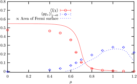
Figure 1: Chiral and diquark condensates as functions of chemical potential.

The data were then extrapolated linearly in $V^{-1}$ to the infinite volume limit. The data are presented as the circular points in Fig. 1. As expected, we see that chiral symmetry is broken at zero chemical potential, as signified by a large chiral condensate, and is approximately restored after the condensate passes through a broad crossover and becomes approximately zero in the high $\mu$ phase. We can also calculate $\left<{\overline{\chi}}\chi\right>$ analytically via a self-consistency equation (the gap equation) in the limit that the number of fermion species (which we rather arbitrarily refer to as the number of colours $N_{c}$) is taken to infinity. This is plotted as the solid curve and can be seen to qualitatively agree with the lattice data, in which the ${\cal O}(1/N_{c})$ corrections are $\approx 15\%$.

In order to explore the possibility of a U(1)_B-violating BCS phase at high $\mu$ we study the relevant order parameter, the diquark condensate $\left<qq_{+}\right>$, which in analogy with the chiral condensate is defined by

$$\left<qq_{+}\right>=\frac{1}{V}\frac{\partial\ln{\cal Z}}{\partial j}=\frac{1}{4V}\left<{\rm tr}\left(\begin{array}[]{c c}\tau_{2}&\\ &\tau_{2}\end{array}\right){\cal A}^{-1}\right>.$$ (5)

Here, the positive subscript highlights the fact that $\left<qq_{+}\right>$ is the sum of contributions from both $\chi\chi$ and $\bar{\chi}\bar{\chi}$ states. This expectation value is measured for ten values of $j$ between 0.1 and 1.0 on the same volumes and with the same parameters with which we measure $\left<{\overline{\chi}}\chi\right>$. Unlike $\left<{\overline{\chi}}\chi\right>$, however, the data are found not to scale with inverse volume, but instead appear to scale linearly with inverse temporal extent. Accordingly, we extrapolate our data to $L_{t}^{-1}\to 0$ corresponding to the zero temperature limit. Some of these data are presented in Fig. 2.

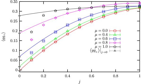
Figure 2: Diquark condensate as a function of $j$ in the zero temperature limit for various $\mu$.

In contrast with the measurement of $\left<{\overline{\chi}}\chi\right>$, in which the bare quark mass is left non-zero as the chiral symmetry of QCD is believed to only ever be approximately conserved, we are required to extrapolate the data for $\left<qq_{+}\right>$ to the $j\to 0$ limit, in which the phenomenologically exact U(1) symmetry related to the conservation of baryon number is restored. By empirically fitting a quadratic curve through the $\mu=0$ data, one finds that as $j$ goes to zero so does $\left<qq_{+}\right>$, implying that there is no condensation in the vacuum as expected. For values of $\mu$ in the chirally restored phase, however, the picture is not quite so clear. It appears that the data correspond to a non-zero diquark condensate, but one can only fit a curve though a subset of the data such that one is required to disregard data with $j\leq 0.2$. Whilst the resulting curves appear to fit the remaining data well, it is important to be able to justify this omission, especially as the data omitted are those closest to limit which one is attempting to reach.

The most obvious possibility is that the condensate is suppressed due to finite volume effects, since diquark condensation is associated with the breaking of a global symmetry; as the symmetry breaking source is reduced to zero, the correlation length $\xi$ of the fluctuations of the order parameter should diverge and become comparable to the size of the lattice.

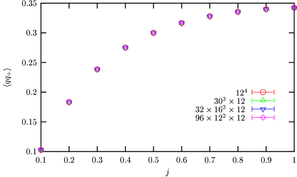
Figure 3: Diquark condensate vs. $j$ at $\mu=0.8$ on $L_{t}=12$ lattices with various spacial volumes.

Figure 3, however, shows some results from an extensive finite volume study, which illustrates that $\left<qq_{+}\right>$ shows little or no change for any value of $j$, even when the spatial volume is altered by a factor of $2.5^{3}\approx 16$. It seems impossible, then, that this is the source of the suppression of the condensate at low $j$. Another possibility is that this suppression is due to having poor control over the extrapolation to zero temperature.

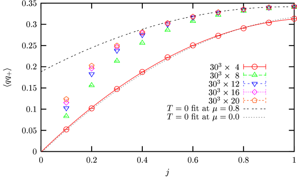
Figure 4: Diquark condensate as a function of $j$ at $\mu=0.8$ at various temperatures.

Figure 4 shows the results of a study of the model at $\mu=0.8$ and with various inverse temporal extents, corresponding to various non-zero temperatures, as well as the curves fitted to $j\in[0.3,1.0]$ of our $\mu=0.0$ and $\mu=0.8$ data after the $T\to 0$ extrapolation. At the highest temperature studied, for which $L_{t}=4$, if one performs a quadratic extrapolation through the data one observes that $\left<qq_{+}\right>=0$ in the $j\to 0$ limit and that the curve closely resembles the $\mu=0.0$ curve at zero temperature. This suggests that although we are within the chirally restored phase, the temperature with $L_{t}=4$ is above the critical temperature for superfluidity for all $j$. As the temperature is decreased (i.e. as the $L_{t}$ is increased to 8) the value of $\left<qq_{+}\right>$ at $j=1.0$ immediately approaches the curve fitted to our zero temperature results, whilst for lower values of $j$ this only occurs at even lower temperatures. This can be understood if one considers the fact that the effect of $j$ is to make the condensate robust not only to finite volume effects, but also to other perturbations such as thermal fluctuations. For a given value of $j$, therefore, there should be some pseudo-critical temperature $T_{c}(j)$ below which the data can be said to be in the superfluid phase, and which in the thermodynamic limit should increase monotonically with $j$. This idea is well illustrated by the data measured on the $30^{3}\times 12$ lattice, shown in Fig. 5.

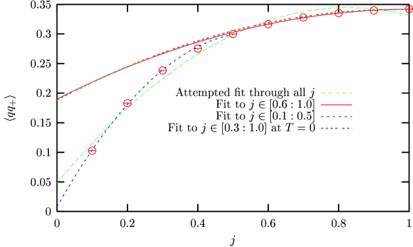
Figure 5: Diquark condensate as a function of $j$ at $\mu=0.8$ on a $30^{3}\times 12$ lattice.

An attempted fit to a single quadratic through all values of $j$ is of very poor quality, whilst by choosing to split the data at some suitable point and fitting the two regions separately, two very reasonable fits can be obtained. In particular, a fit to the data with $j\leq 0.5$ is consistent with $\left.\left<qq_{+}\right>\right|_{j\to 0}=0$ suggesting that for these values of $j$, $L_{t}=12$ is above the pseudo-critical temperature. The fit to the data with $j\geq 0.6$, however, is consistent with $\left.\left<qq_{+}\right>\right|_{j\to 0}\neq 0$ and agrees almost exactly with the fit to data from the $12^{4}$, $16^{4}$ and $20^{4}$ lattices extrapolated to $T\to 0$ and then $j\in[0.3,1.0]\to 0$, suggesting that this curve represents the true zero temperature limit and justifies our discarding of data with $j\leq 0.2$. Whilst a linear $T\to 0$ extrapolation is sufficient to reach this curve for $0.3\leq j\leq 0.5$, the condensate at $j<0.3$ must be suppressed too much for such an extrapolation to be sufficient, i.e. the temperature of the lattice on our three lattice volumes must be too high compared with $T_{c}(j<0.3)$.

Finally, now that we can trust our $T\to 0$ and $j\to 0$ extrapolations, let us look back at Fig. 1, where the diquark condensate is plotted with the chiral condensate as a function of $\mu$. Although there is clearly a transition from a phase with no diquark condensation to one in which the diquark condensate has a magnitude similar to that of the vacuum chiral condensate, this transition is far less pronounced than in the chiral case. $\left<qq_{+}\right>$ increases approximately as $\mu^{2}$, but eventually saturates as $\mu$ approaches 1.0 and even decreases past $\mu\sim 1.1$. This behaviour is directly related to the geometry of the Fermi surface for a system defined on a cubic lattice, the area of which we can calculate in the large-$N_{c}$ free fermion limit and is plotted as the dashed curve. In the continuum, therefore, $\left<qq_{+}\right>$ should continue to rise as $\mu^{2}$.

IV Measurement of the gap

In the previous section, we presented evidence for superfluidity in the form of a non-zero diquark condensate at high chemical potential. Here we present more direct evidence for a superfluid phase by mapping out the fermion dispersion relation (i.e. the energy $E$ as a function of momentum $k$) and observing a BCS energy gap $\Delta$ about the Fermi momentum. One advantage of this order parameter over the diquark condensate is that it is directly related to a macroscopic property of the superfluid, the critical temperature $T_{c}$ Schmitt et al. (2002). Also, being a global order parameter, in principle it would be possible to measure in a gauge theory such as QCD, where according to Elitzur’s theorem, one cannot write down a local order parameter such as $\left<qq_{+}\right>$ in a gauge invariant way Elitzur (1975).

In order to extract the dispersion relation we define the time-slice propagator

$${\cal G}(\vec{k};t)=\sum_{\vec{x}}{\cal G}(\vec{0},0;\vec{x},t)e^{-i\vec{k}.\vec{x}},$$ (6)

where

$${\cal G}(x;y)={\cal A}^{-1}_{xy}=\left(\begin{array}[]{c c}A_{xy}&N_{xy}\\ \bar{N}_{xy}&\bar{A}_{xy}\end{array}\right)$$ (7)

is the Gor’kov propagator. As in the original BCS theory Bardeen et al. (1957), the fermionic degrees of freedom can be viewed as quasi-particles with energy $E$ relative to the system’s Fermi energy $E_{F}$. In the limit that $j\to 0$, the propagation of these quasi-particles is described by the “normal” $\left<q(0)\overline{q}(x)\right>$ and $\left<\overline{q}(0)q(x)\right>$ parts of (6), i.e. those that are off-diagonal in the Nambu-Gor’kov space and related to $M^{-1}$. If the Fermi surface is unstable with respect to a BCS ground-state, the quasi-particles nearest to $E_{F}$ undergo particle-hole mixing and a gap appears in the energy spectrum. The propagation of these mixed states is generated by the diagonal, or “anomalous” $\left<q(0)q(x)\right>$ and $\left<\overline{q}(0)\overline{q}(x)\right>$ parts of (6). By a combination of symmetry constraints and empirical observations we note that the complex matrix ${\cal G}(\vec{k},t)$ contains only two independent parts, one in $\bar{N}_{xy}$ and one in $A_{xy}$, which from hereon shall be referred to simply as the normal and anomalous propagators and written as $N(k,t)$ and $A(k,t)$ respectively.

We measure $N(k,t)$ and $A(k,t)$ at $\mu=0.8$ on lattices with $L_{x}\times L_{y}\times L_{z}=96\times 12\times 12$ and $L_{t}=16$, $20$ and $24$ using standard lattice techniques and extrapolate linearly in $L_{t}^{-1}$ to zero temperature. This choice means that by choosing $\vec{k}=(k,0,0)$ in (6) we can study 25 independent momentum modes in the $x$ direction between 0 and $\pi/{2a}$. We may then extract the energy by fitting them to

$$\begin{array}[]{c l l}N(k,t)=Ae^{-Et}+Be^{-E(L_{t}-t)}&{\rm if}&t={\rm odd}\\ N(k,t)=0&{\rm if}&t={\rm even}\end{array}$$ (8)

and

$$\begin{array}[]{c l l}A(k,t)=C(e^{-Et}-e^{-E(L_{t}-t)})&{\rm if}&t={\rm even}\\ A(k,t)=0&{\rm if}&t={\rm odd},\end{array}$$ (9)

where $A$, $B$ and $C$ are kept as free parameters, as is the energy $E$, which as expected is found to be the same from both (8) and (9). These parameters are then, in turn, extrapolated to $j\to 0$. Quadratic polynomial curves are fitted to the coefficients $A(k)$, $B(k)$ and $C(k)$, whilst the energy $E(k)$ is fitted with a straight line. As with the extrapolation of $\left<qq_{+}\right>$ in the previous section, the extrapolations appear to smoothly fit the data except for at low $j$, where the discrepancy we have attributed to non-zero temperature persists. Again, for the purpose of the extrapolations, we believe we are justified in ignoring points with $j<0.3$.

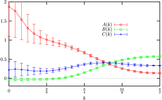
Figure 6: Propagator coefficients $A$, $B$ and $C$ at $\mu=0.8$ in the zero temperature and source limits.

Figure 6 shows the coefficients of the normal and anomalous propagators, after the extrapolations to zero temperature and diquark source, plotted as functions of momentum $k$. Since the normal propagator was chosen from the $\bar{N}_{xy}$ part of ${\cal G}$, the forward moving signal proportional to the coefficient $A(k)$ relates to the propagation of holes in the Fermi sea, whilst the backward moving signal proportional to $B(k)$ relates to the propagation of particle excitations above the Fermi surface. Accordingly, we see that the low momentum excitations near the centre of the Fermi sphere are dominated by hole degrees of freedom, whilst the high momentum excitations are dominated by particles. To excitations at the Fermi surface, the propagation of fermions forward and backward in time should be equal, such that the point where $A(k)$ and $B(k)$ cross allows us to define the Fermi momentum $k_{F}$. The coefficient $C(k)\sim 0$ at low momentum, but becomes non-zero in a broad peak about the position of $k_{F}$. This vanishing of the anomalous propagator $A(k,t)$, even in the limit that $j\to 0$ is a signal of particle-hole mixing in the presence of a BCS gap.

For more direct evidence, let us look at the left panel of Fig. 7, which shows the dispersion relation at $\mu=0.8$ and again extrapolated to $T\to 0$ and $j\in[0.3,1.0]\to 0$.

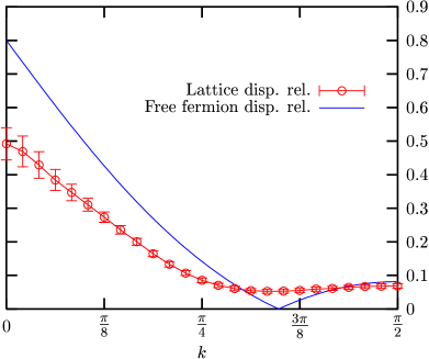
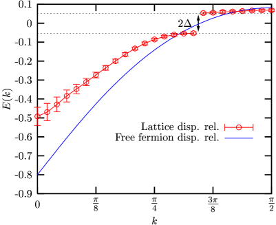
Figure 7: The lattice dispersion relation and typical free fermion dispersion relation at $\mu=0.8$. In the right-hand panel the hole branch is plotted as negative.

The solid curve shows the dispersion relation for free massless staggered fermions, which has two distinct branches, the hole branch where $E(k)$ decreases with $k$ corresponding to excitations below $E_{F}$ and the particle branch where $E(k)$ increases with $k$ corresponding to excitations above $E_{F}$. In contrast to this, the dispersion relation from our lattice data shows no discontinuity between the two branches, which is another sign of particle-hole mixing. More importantly, at no time does the curve pass through $E=0$ as there is a distinct gap between this point and the minimum; this is the BCS gap $\Delta=0.053(6)$. This can be seen in a more familiar light if we plot the hole branch as negative, as illustrated in the right-hand panel of Fig. 7. This makes the free fermion dispersion relation a smooth continuous curve, as one would expect, whilst for the NJL dispersion relation this introduces a discontinuity at $k_{F}$, which gives a clear illustration of the BCS gap. In order to present the value of the gap as a dimensionless ratio, we also measure the fermion mass at $\mu=0$ from the vacuum dispersion relation which gives us

$$\frac{\Delta(\mu=0.8)}{\Sigma(\mu=0.0)}=0.15(2).$$ (10)

Assuming a fermion mass of 400MeV, this implies that $\Delta(\mu=0.8)\approx 60{\rm MeV}$, consistent with the analytic predictions of Berges and Rajagopal (1999); Nardulli (2002).

Finally, in order to investigate the $\mu$ dependence of $\Delta$, we determine dispersion relations for a range of chemical potentials in $0.50\leq\mu\leq 0.85$, this time using data from $L_{t}=16$ and 20 only. Whilst this means that the extrapolation to $T=0$ is no longer an overdetermined problem and requires one to estimate the error, it is worth noting that the resulting dispersion relation at $\mu=0.8$ agrees with that presented in Fig. 7 for all $k$.

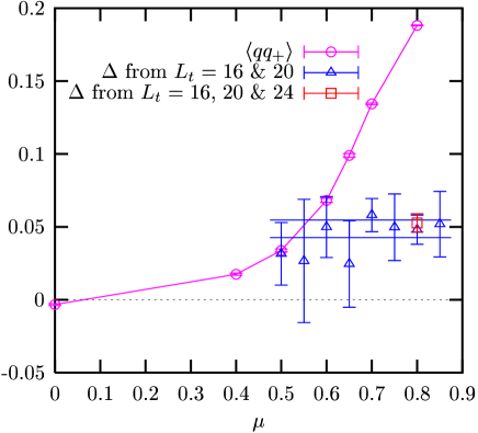
Figure 8: The gap $\Delta$ as a function of $\mu$ compared with $\left<qq_{+}\right>$

By calculating $E(k)$ and extracting the minimum, we are able to plot $\Delta(\mu)$ in Fig. 8, where it is compared with the diquark condensate $\left<qq_{+}\right>$. Whilst the condensate rises with $\mu$, the gap shows no evidence of any $\mu$ dependence in the chirally restored phase and a least-squares fit to $\Delta=constant$ has a $\chi^{2}$ of only 0.33 per degree of freedom. In combination with Fig. 1, this supports the simple-minded picture in which only quark pairs within a shell about $E_{F}$ of thickness $2\Delta$, independent of $\mu$, contribute to diquark condensation, resulting in a condensate $\left<qq_{+}\right>\propto\Delta\mu^{2}$.

V Summary

In this talk we have seen evidence, first presented in Hands and Walters (2004), for a BCS superfluid phase at high $\mu$ and low $T$ in the $3+1d$ lattice NJL model in the form of a non-vanishing local order parameter and, for the first time in the systematic study of a relativistic field theory, a direct observation of a BCS gap. Given that the model shares its global symmetries with the real world, we believe that we are justified in treating this as phenomenological evidence for the existence of a similar colour superconducting phase in full QCD.

Appendix A The lattice Fermi surface

The conclusions drawn from Figs. 3 and 5 (i.e. that $\left<qq_{+}\right>$ is approximately independent of spatial volume and that one would need to use $L_{t}\gg 20$ to reproduce the curves in Fig. 2 without discarding any data) might suggest that one could successfully reach the zero temperature limit quite cheaply by performing simulations with $L_{t}\gg L_{s}$. For this reason it is worth making the cautionary point that performing simulations with $\mu\neq 0$ on such lattices can lead to unexpected results. At low temperature, the Fermi-Dirac distribution resembles a step function, with the discontinuity about the Fermi momentum smeared out across a region $\delta k\sim T\sim L_{t}^{-1}$; in a finite system, the Brillouin zone is discretised into a cubic momentum lattice with lattice spacing $2\pi/(aL_{s})$. For lattices with $L_{t}\gg L_{s}$, therefore, the smearing of the Fermi surface is too fine to be resolved on the coarse momentum lattice. One consequence is that when the chemical potential is increased smoothly, the Fermi-Dirac distribution changes only when the Fermi surface crosses a momentum mode. If one were to study a transition, therefore, such as the chiral crossover illustrated in Fig. 1, the physics of the system would be approximately constant except at points where the surface crosses a mode; the transition would be turned into a series of steps.

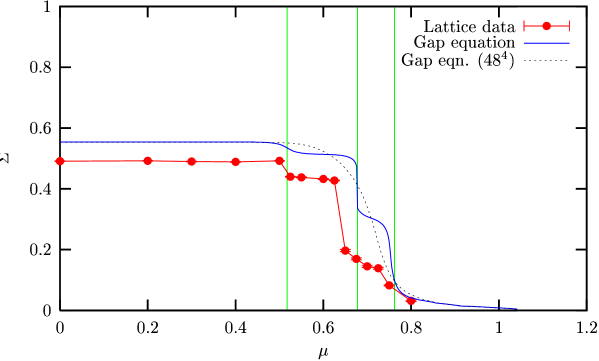
Figure 9: Expectation value of the scalar field vs. $\mu$ on a $10^{3}\times 48$ lattice.

This is nicely illustrated in Fig. 9, where the expectation value of the scalar field $\Sigma\equiv\left<\sigma\right>$ is plotted as a function of $\mu$ on a $10^{3}\times 48$ lattice. The Solid curve is $\Sigma$ solved via the gap equation in the large-$N_{c}$ limit and can be seen to change significantly only when the solutions of the free-Fermion dispersion relation in the infinite volume limit

$$\mu\sim E_{F}=\sqrt{\sum_{i=1}^{3}\sin^{2}{k_{F}}_{i}+\Sigma^{2}}$$ (11)

coincide with one of the lattice momenta. The first three of these points are denoted by the vertical lines. The lattice data agree qualitatively with this curve and the discontinuities can be seen clearly. For this reason one cannot make the ratio $L_{t}/L_{s}$ arbitrarily large.

References

- Rajagopal and Wilczek (2001) K. Rajagopal and F. Wilczek, Handbook of QCD (World Scientific, 2001), chap. 35.
- Rischke (2004) D. H. Rischke, Prog. Part. Nucl. Phys. 52, 197 (2004).
- Berges and Rajagopal (1999) J. Berges and K. Rajagopal, Nucl. Phys. B538, 215 (1999).
- Alford et al. (1999) M. G. Alford, K. Rajagopal, and F. Wilczek, Nucl. Phys. B537, 443 (1999).
- Hands et al. (2000) S. J. Hands et al., Eur. Phys. J. C17, 285 (2000).
- Aloisio et al. (2001) R. Aloisio, V. Azcoiti, G. Di Carlo, A. Galante, and A. F. Grillo, Nucl. Phys. B606, 322 (2001).
- Kogut et al. (2001) J. B. Kogut, D. K. Sinclair, S. J. Hands, and S. E. Morrison, Phys. Rev. D64, 094505 (2001).
- Hands et al. (2001) S. J. Hands, I. Montvay, L. Scorzato, and J. Skullerud, Eur. Phys. J. C22, 451 (2001).
- Nambu and Jona-Lasinio (1961) Y. Nambu and G. Jona-Lasinio, Phys. Rev. 122, 345 (1961).
- Hands and Walters (2004) S. J. Hands and D. N. Walters, Phys. Rev. D69, 076011 (2004).
- Hands et al. (2002) S. J. Hands, B. Lucini, and S. E. Morrison, Phys. Rev. D65, 036004 (2002).
- Klevansky (1992) S. P. Klevansky, Rev. Mod. Phys. 64, 649 (1992).
- Schmitt et al. (2002) A. Schmitt, Q. Wang, and D. H. Rischke, Phys. Rev. D66, 114010 (2002).
- Elitzur (1975) S. Elitzur, Phys. Rev. D12, 3978 (1975).
- Bardeen et al. (1957) J. Bardeen, L. N. Cooper, and J. R. Schrieffer, Phys. Rev. 108, 1175 (1957).
- Nardulli (2002) G. Nardulli, Riv. Nuovo Cim. 25N3, 1 (2002).