Finite volume effects using lattice chiral perturbation theory

Abstract

Lattice regularization is used to perform chiral perturbation theory calculations in finite volume. The lattice spacing is chosen small enough to be irrelevant, and numerical results are obtained from simple summations.

1 CONTEXT

Lattice QCD simulations are necessarily performed in a finite volume though one is typically interested in results for infinite spacetime. The extrapolation introduces a systematic uncertainty which needs to be controlled. As the lightest particle in the QCD spectrum, the pion has a large Compton wavelength and therefore plays a key role in these volume effects, so chiral perturbation theory is the natural tool for studying volume dependences. After the pioneering work of Gasser and Leutwyler[1], there has been a lot of activity on this topic. Some recent studies in the light meson sector can be found in Refs. [2, 3, 4, 5].

Physical results do not depend on regularization scheme. For chiral perturbation theory in a finite volume, lattice regularization is numerically convenient because loop diagrams are finite summations for any nonzero lattice spacing. Divergences would appear as the lattice spacing vanishes, but for the volume effects studied here we can simply use a nonzero lattice spacing which is small enough to be numerically irrelevant.

The present work uses the lattice regularized chiral perturbation theory Lagrangian of Ref. [6], but for two flavors rather than three. Extra $O(a)$ terms could be added to the Lagrangian but they are irrelevant in the continuum limit, and our present goal is the computation of finite volume effects for the continuum limit.

2 THE PION MASS

Figure 1: One-loop Feynman diagrams for the pion mass.

Consider an isotropic spacetime lattice with spacing “$a$”, $N_{s}$ sites in each spatial direction and $N_{t}$ sites in the temporal direction. The pion mass is obtained at the one-loop level from the diagrams in Fig. 1. The propagators and vertices are obtained from the Lagrangian of Ref. [6] in a straightforward manner, and loop momenta are summed. The resulting Green’s function is

$$\Gamma = \Gamma_{\rm LO}+\Gamma_{\rm NLO}^{(a)}+\Gamma_{\rm NLO}^{(b)},$$ (1)

$$\Gamma_{\rm LO} = -x_{\pi}^{2}-\frac{2}{a^{2}}\sum_{\mu}(1-\cos ap_{\mu}),$$ (2)

$$\Gamma_{\rm NLO}^{(a)} = -\frac{2}{3a^{4}F^{2}}-\frac{2x_{\pi}^{4}}{F^{2}}(l_{3}+l_{4})$$ (3)

$$-\frac{2l_{4}x_{\pi}^{2}}{a^{2}F^{2}}\sum_{\mu}\sin^{2}ap_{\mu},$$

$$\Gamma_{\rm NLO}^{(b)} = \frac{1}{6N_{s}^{3}N_{t}a^{4}F^{2}}\sum_{k}\bigg{(}112+5a^{2}x_{\pi}^{2}$$ (4)

$$-20\sum_{\mu}\cos ap_{\mu}-20\sum_{\mu}\cos ak_{\mu}$$

$$\left.+12\sum_{\mu}\cos ap_{\mu}\cos ak_{\mu}\right)D(k),$$

where

$$D(k)=\frac{1}{a^{2}x_{\pi}^{2}+2\sum_{\mu}(1-\cos ak_{\mu})}$$ (5)

is the pion propagator and

$$x_{\pi}=\sqrt{2Bm_{q}}$$ (6)

is the lowest-order pion mass in the continuum limit. (We work in the isospin limit, $m_{q}\equiv m_{u}=m_{d}$.) The momentum summations include $k_{1,2,3}=\frac{2\pi n}{aN_{s}}$ with $n=1,2,3,\ldots N_{s}$ and $k_{4}=\frac{2\pi n}{aN_{t}}$ with $n=1,2,3,\ldots N_{t}$.

The pion mass is obtained by solving $\Gamma=0$ for $ip_{4}$ with $\vec{p}=0$. The result is

$$M_{\pi} = \frac{2}{a}{\rm arcsinh}\left(\frac{aX_{\pi}}{2}\right),$$ (7)

$$X_{\pi}^{2} = x_{\pi}^{2}+\frac{2x_{\pi}^{4}l_{3}}{F^{2}}$$ (8)

$$+x_{\pi}^{2}\sum_{k}\frac{(3-2\cos ak_{4})}{2N_{s}^{3}N_{t}a^{2}F^{2}}D(k)+O(a).$$

Having simply written down the pion mass in terms of Feynman vertices and propagators, we can now do the summation numerically to obtain the pion mass. The numerical values of the parameters $x_{\pi}$ and $l_{3}$ will depend sensitively on lattice spacing since they must absorb terms that diverge as $a\to 0$. Nevertheless the computation is finite for any $a\neq 0$, and for sufficiently small $a$ the observable pion mass is independent of $a$.

To study spatial volume effects on a lattice of infinite temporal extent, we can choose $N_{t}\gg N_{s}$ and compute the difference of $M_{\pi}$ at two different spatial volumes. In this computation, the $l_{3}$ term and the leading $x_{\pi}^{2}$ term and all “would-be divergences” subtract away. The resulting computation of volume dependence is plotted in Fig. 2. By choosing $a=0.1$ fm, $N_{t}=5N_{s}$ and approximating an infinite volume by $L_{s}=8$ fm, the numerical results are found to agree with the standard one-loop results discussed, for example, in Ref. [3]. Figure 2 also shows the errors that would arise by increasing $a$, decreasing $N_{t}$ or decreasing the approximation to infinite spatial length.

It is clear from the simplicity of Eq. (8) that the computation is inexpensive.

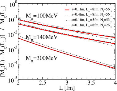
Figure 2: Volume effects for the pion mass.

3 OTHER PION OBSERVABLES

Figure 3: One-loop Feynman diagrams for the pion decay constant.

Figure 4: One-loop Feynman diagrams for the pion form factor.

Other observables can be computed similarly. The Feynman diagrams for the pion decay constant and form factor are shown in Figs. 3 and 4 respectively, where $Z$ denotes wave function renormalization and is obtained from Eq. (1) in the usual way. Writing down the vertices and propagators of Figs. 3 and 4 with a summation over each loop momentum leads directly to finite expressions that can be computed numerically. The volume dependences of the decay constant, form factor and charge radius (obtained by differentiating the form factor) are shown in Figs. 5, 6 and 7 respectively. Results for the decay constant agree with the one-loop calculation of Ref. [4]. Notice that the charge radius has a large fractional dependence on volume since loop effects occur at leading order for this observable.

Acknowledgements

This work was supported in part by Deutsche Forschungsgemeinschaft, the Natural Sciences and Engineering Research Council of Canada, and the Canada Research Chairs Program.

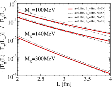
Figure 5: Volume effects for the pion decay constant.

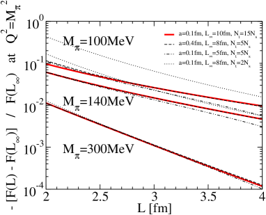
Figure 6: Volume effects for the pion form factor.

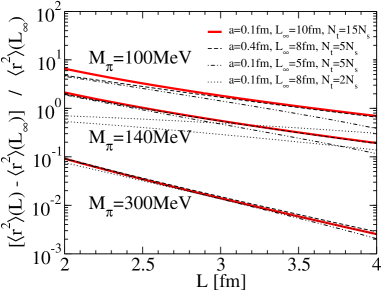
Figure 7: Volume effects for the pion charge radius.

References

- [1] J. Gasser and H. Leutwyler, Nucl. Phys. B307, 763 (1988).
- [2] M.F.L. Golterman, K.C. Leung, Phys. Rev. D56, 2 (1997); M. Golterman, E. Pallante, Nucl. Phys. (Proc. Suppl.) 83, 250 (2000); C.J.D. Lin, G. Martinelli, E. Pallante, C.T. Sachrajda, G. Villadoro, Phys. Lett. B553, 229 (2003); D. Becirevic, G. Villadoro, Phys. Rev. D69, 054010 (2004).
- [3] G. Colangelo, S. Durr, Eur. Phys. J. C33, 543 (2004).
- [4] G. Colangelo, C. Haefeli, hep-lat/0403025.
- [5] G. Colangelo, these proceedings.
- [6] R. Lewis, P.-P.A. Ouimet, Phys. Rev. D64, 034005 (2001); B. Borasoy, R. Lewis, P.-P.A. Ouimet, Phys. Rev. D65, 114023 (2002).