Abstract

We compute the $1$-loop chiral corrections to the bag parameters which are needed for the discussion of the SUSY $K^{0}\!-\!{\overline{K^{0}}}$ mixing problem in both finite and infinite volume. We then show how the bag parameters can be combined among themselves and with some auxiliary quantities and thus sensibly reduce the systematic errors due to chiral extrapolations as well as those due to finite volume artefacts that are present in the results obtained from lattice QCD. We also show that in some cases these advantages remain as such even after including the $2$-loop chiral corrections. Similar discussion is also made for the $K\to\pi$ electro-weak penguin operators.

1 Introduction

We are entering the era of the large scale unquenched numerical simulations of QCD on the lattice and so the error on the $B_{K}$ parameter, currently dominated by the systematic error due to quenching [1], is likely to fall below $10$% quite soon. This will further improve our knowledge on the shape of the CKM unitarity triangle [2], i.e., on the value of the CKM phase which is responsible for all the CP-violating phenomena in the Standard Model (SM). Since the CP-violation in SM is too small to explain the dynamical generation of the baryon asymmetry of the Universe [3], one is tempted to look for additional sources of CP-violation beyond the SM. Supersymmetric (SUSY) extensions of the SM, besides providing an elegant solution to the hierarchy problem, also provide new CP-violating phases whose size can be constrained by the experimentally measured processes governed by the flavor changing neutral currents (FCNC). A convenient way to study those is by using the mass insertion approximation [4]. In the basis in which the couplings of quarks and squarks to the neutral gauginos are flavor diagonal, the flavor changing insertions arise from the small off-diagonal terms in the squark masses, parameterized by dimensionless complex parameters

$$(\delta^{u/d}_{ij})_{AB}={(\Delta_{ij}^{u/d})_{AB}\over m_{\tilde{q}}^{2}}\,,$$ (1)

where $m_{\tilde{q}}$ is the diagonal squark mass (averaged as $m_{\tilde{q}}=\sqrt{m_{\tilde{q}_{i}}m_{\tilde{q}_{j}}}$), and $(\Delta_{ij}^{u/d})_{AB}$ are the off-diagonal elements which mix both the left-handed and right-handed squark flavors ($i,j=1,2,3$; $A,B=L,R$). Like in the SM, $\varepsilon_{K}$, the parameter which measures the indirect CP-violation in the neutral kaon system, is given by

$$\varepsilon_{K}={{\rm Im}\langle K^{0}|{\cal H}^{\Delta S=2}_{\rm eff}|\bar{K}^{0}\rangle\over\Delta m_{K}\;\sqrt{2}}\,,$$ (2)

but unlike in the SM, the effective Hamiltonian in SUSY [${\cal H}^{\Delta S=2}_{\rm eff}=\sum_{i}C_{i}(\mu)O_{i}(\mu)$], besides the left-left ($LL$) four-quark operator, also contains the $LR$, $RL$ and $RR$ ones (see below for the specific bases of such operators). The Wilson coefficients, $C_{i}(\mu)$, can be computed perturbatively in any specific low energy SUSY model. The matrix elements, instead, must be computed non-perturbatively. To date the most suitable tool to do such a computation is by means of lattice QCD. The matrix elements of the non-SM operators are enhanced with respect to the SM one by a large factor, $m_{K}^{2}/(m_{s}+m_{d})^{2}\approx 25$, and therefore their more accurate determination is mandatory. So far these matrix elements have been computed in quenched lattice QCD by considering kaons consisting of degenerate quarks [5]. The corresponding results are then used to discuss the constraints on $(\delta^{d}_{12})_{AB}$ [6], along the lines proposed in ref. [7]. In addition to unquenching, the lattice estimates should be improved by fixing one of the kaons’ valence quarks to the physical strange quark mass (accessible in the lattice simulations) and pushing the other one as close to the chiral limit as possible. Due to limited computing resources, however, two problems appear: (1) one cannot work with the light quark as light as the physical $d$-quark and therefore a chiral extrapolation will always be needed; (2) the finite volume effects become more pronounced as the light quark mass is decreased. In such a situation and in order to get the phenomenologically interesting results from lattice QCD on the matrix elements relevant to the SUSY $K^{0}\!-\!{\overline{K^{0}}}$ mixing problem, one should find a way to reduce uncertainties related to these two problems. In this paper these issues are addressed and further considered by using chiral perturbation theory (ChPT). We compute the chiral logarithmic corrections to the so called “bag”-parameters and discuss the possible strategies that would allow one to minimize their impact onto the chiral extrapolations of the lattice results, as well as to minimize the systematic errors due to finite volume. In Sec. 2 we recall the frequently employed bases of $\Delta S=2$ operators and define the bag-parameters, to which we compute the chiral corrections in Sec. 3. In Sec. 4 we discuss the combinations of bag parameters which are (completely or partially) free of chiral logarithms, and we briefly comment (Sec. 5) on the application of a similar strategy to the $K\to\pi$ matrix elements that are relevant to the $\Delta I=3/2$ amplitude in $K\to\pi\pi$ decay. In Sec. 6 we discuss the impact of the $2$-loop chiral corrections to one class of the combinations of bag parameters, and we briefly conclude in Sec. 7.

2 Bases of $\Delta S=2$ operators and $B$-parameters

The SUSY contributions to the $K^{0}\!-\!{\overline{K^{0}}}$ mixing amplitude are usually discussed in the so called SUSY basis of $\Delta S=2$ operators [7]:

$${\phantom{{l}}}\raisebox{-4.55254pt}{\phantom{{j}}}O_{1} = \ \bar{s}^{i}\gamma_{\mu}(1-\gamma_{5})d^{i}\,\bar{s}^{j}\gamma_{\mu}(1-\gamma_{5})d^{j}\,,$$

$${\phantom{{l}}}\raisebox{-4.55254pt}{\phantom{{j}}}O_{2} = \ \bar{s}^{i}(1-\gamma_{5})d^{i}\,\bar{s}^{j}(1-\gamma_{5})d^{j}\,,$$

$${\phantom{{l}}}\raisebox{-4.55254pt}{\phantom{{j}}}O_{3} = \ \bar{s}^{i}(1-\gamma_{5})d^{j}\,\bar{s}^{j}(1-\gamma_{5})d^{i}\,,$$ (3)

$${\phantom{{l}}}\raisebox{-4.55254pt}{\phantom{{j}}}O_{4} = \ \bar{s}^{i}(1-\gamma_{5})d^{i}\,\bar{s}^{j}(1+\gamma_{5})d^{j}\,,$$

$${\phantom{{l}}}\raisebox{-4.55254pt}{\phantom{{j}}}O_{5} = \ \bar{s}^{i}(1-\gamma_{5})d^{j}\,\bar{s}^{j}(1+\gamma_{5})d^{i}\,,$$

where the superscripts stand for the color indices. Other bases are also employed, of which the Dirac basis is probably the most popular among the lattice QCD practitioners,

j $$Q_{1}=\bar{s}^{i}{\gamma}_{\mu}(1-{\gamma}_{5})d^{i}\ \bar{s}^{j}{\gamma}_{\mu}(1-{\gamma}_{5})d^{j}\;,$$

j $$Q_{2}=\bar{s}^{i}{\gamma}_{\mu}(1-{\gamma}_{5})d^{i}\ \bar{s}^{j}{\gamma}_{\mu}(1+{\gamma}_{5})d^{j}\;,$$

j $$Q_{3}=\bar{s}^{i}(1+{\gamma}_{5})d^{i}\ \bar{s}^{j}(1-{\gamma}_{5})d^{j}\;,$$ (4)

j $$Q_{4}=\bar{s}^{i}(1-{\gamma}_{5})d^{i}\ \bar{s}^{j}(1-{\gamma}_{5})d^{j}\;,$$

j $$Q_{5}=\bar{s}^{i}\sigma_{\mu\nu}d^{i}\ \bar{s}^{j}\sigma_{\mu\nu}d^{j}\;,$$

where we use the definition in which $\sigma_{\mu\nu}=[\gamma_{\mu},\gamma_{\nu}]/2$. Although the operators in the above bases are written with both parity even and parity odd parts, only the parity even ones survive in the kaon matrix elements. The latter are usually parameterized in terms of bag-parameters $B_{{1}{\mathrm{-}}{5}}$, namely,

$$\langle\bar{K}^{0}|O_{1}(\nu)|K^{0}\rangle = {8\over 3}\,m_{K}^{2}f_{K}^{2}\ B_{1}(\nu)\ ,$$

$$\langle\bar{K}^{0}|O_{2}(\nu)|K^{0}\rangle = -{5\over 3}\,\left({m_{K}\over m_{s}(\nu)+m_{d}(\nu)}\right)^{2}m_{K}^{2}f_{K}^{2}\ B_{2}(\nu)\,,$$

$$\langle\bar{K}^{0}|O_{3}(\nu)|K^{0}\rangle = {1\over 3}\,\left({m_{K}\over m_{s}(\nu)+m_{d}(\nu)}\right)^{2}m_{K}^{2}f_{K}^{2}\ B_{3}(\nu)\,,$$ (5)

$$\langle\bar{K}^{0}|O_{4}(\nu)|K^{0}\rangle = 2\,\left({m_{K}\over m_{s}(\nu)+m_{d}(\nu)}\right)^{2}m_{K}^{2}f_{K}^{2}\ B_{4}(\nu)\,,$$

$$\langle\bar{K}^{0}|O_{5}(\nu)|K^{0}\rangle = {2\over 3}\,\left({m_{K}\over m_{s}(\nu)+m_{d}(\nu)}\right)^{2}m_{K}^{2}f_{K}^{2}\ B_{5}(\nu)\,,$$

where $B_{i}>0$. $\nu$ in the above equation indicates the renormalization scale of the logarithmically divergent operators, $O_{i}$, and the scale at which the separation between the long-distance (matrix elements) and short-distance (Wilson coefficients) physics is made. To make contact between the matrix elements of the operators in (2) and those in (2), one applies the Fierz identity on the Dirac structures (FD), which leaves the physical amplitude invariant, and then reorder the color reversed indices in operators $O_{3}$ and $O_{5}$. For example,

$$\langle\bar{K}^{0}|O_{3}|K^{0}\rangle\equiv\langle O_{3}\rangle=\langle O_{3}^{FD}\rangle=\langle\bar{s}^{i}_{\alpha}d^{j}_{\beta}\bar{s}^{j}_{\gamma}d^{i}_{\delta}\ \left[{11}\otimes{11}+\gamma_{5}\otimes\gamma_{5}\right]^{FD}_{\alpha\beta,\gamma\delta}\rangle=$$

$$-\frac{1}{2}\langle\bar{s}^{i}_{\alpha}d^{i}_{\delta}\bar{s}^{j}_{\gamma}d^{j}_{\beta}\ \left[{11}\otimes{11}+\gamma_{5}\otimes\gamma_{5}-\sigma_{\mu\nu}\otimes\sigma_{\mu\nu}\right]_{\alpha\delta,\gamma\beta}\rangle=\frac{1}{2}\left(\langle Q_{5}\rangle-\langle Q_{4}\rangle\right)\,.$$ (6)

Similarly, $\langle O_{5}\rangle=-(1/2)\langle Q_{2}\rangle$. Summarizing,

$$\langle Q_{1}\rangle=\langle O_{1}\rangle\;,\hskip 31.29802pt\langle Q_{2}\rangle=-2\langle O_{5}\rangle\;,$$ (7)

(8)

$$\langle Q_{3}\rangle=\langle O_{4}\rangle\;,\hskip 31.29802pt\langle Q_{4}\rangle=\langle O_{2}\rangle\;,$$ (9)

(10)

$$\langle Q_{5}\rangle=\langle O_{2}\rangle+2\langle O_{3}\rangle\;.$$ (11)

In eqs. (2,7) and in the rest of this paper the $\nu$-dependence is implicit. As a side remark, we note that these formulae are strictly true only in the renormalization schemes in which the Dirac Fierz identity is not violated, such as the (Landau) ${\rm RI/MOM}$ scheme [8].  In the following we will suppose that the subtraction of ultraviolet divergences is made in such a renormalization scheme and restrict our attention to the low energy behavior of the above matrix elements.

3 Chiral logarithmic corrections

As mentioned in introduction, we will use ChPT to discuss the low energy behavior of $\Delta S=2$ operators relevant to the SUSY $K^{0}\!-\!{\overline{K^{0}}}$ mixing amplitude. Even before considering the chiral representation of eq. (2) or eq. (2), it is clear that the chiral behavior of the matrix elements of $O_{2}$ and $O_{3}$ will be the same since these two operators differ only in the color indices. In other words these two operators differ by a gluon exchange, which is a local effect, that cannot influence the long distance behavior described by ChPT. Therefore the chiral logarithms in $B_{2}$ and $B_{3}$ will be the same although their respective low energy constants (LEC’s) are different. The same argument applies to $B_{4}$ and $B_{5}$. This “color blindness” is evident when working out the chiral representation of the operators (2). To that end, we will use the lagrangian and notation specified in our previous paper [10], and account for the following properties:

• Under ${\rm SU(3)_{L}}\otimes{\rm SU(3)_{R}}$ the field $\Sigma$ transforms as $\Sigma\to R\Sigma L^{\dagger}$;

• The lowest order Lorentz scalars, transforming as $(\bar{3},3)$ and $(3,\bar{3})$, are $\Sigma$ and $\Sigma^{\dagger}$, respectively;

• The lowest order Lorentz vectors, transforming as $(8,1)$ and $(1,8)$, are $i\Sigma^{\dagger}\partial_{\mu}\Sigma$ and $i\Sigma\partial_{\mu}\Sigma^{\dagger}$, respectively.

We are now able to write the bosonised versions of eq. (2), namely,

j $$Q_{1}=-b_{1}\frac{f^{4}}{8}\left(\Sigma^{\dagger}\partial^{\mu}\Sigma\right)_{ds}\left(\Sigma^{\dagger}\partial_{\mu}\Sigma\right)_{ds}\;,$$

j $$Q_{2}=-b_{2}\frac{f^{4}}{4}B_{0}^{2}\Sigma^{\dagger}_{ds}\Sigma_{ds}\;,$$

j $$Q_{3}=b_{3}\frac{f^{4}}{8}B_{0}^{2}\Sigma^{\dagger}_{ds}\Sigma_{ds}\;,$$ (12)

j $$Q_{4}=b_{4}\frac{f^{4}}{8}B_{0}^{2}\left(\Sigma_{ds}\Sigma_{ds}+\Sigma^{\dagger}_{ds}\Sigma^{\dagger}_{ds}\right)\;,$$

j $$Q_{5}=-b_{5}\frac{f^{4}}{8}B_{0}^{2}\left(\Sigma_{ds}\Sigma_{ds}+\Sigma^{\dagger}_{ds}\Sigma^{\dagger}_{ds}\right)\;,$$

where we introduced the new set of bag parameters, $b_{i}$, with the signs chosen as to make all $b_{i}$’s positive. After sandwiching the above operators by $\langle\bar{K}^{0}|$ and $|K^{0}\rangle$ and after evaluating the matrix elements at leading order, we can relate $b_{i}$’s to the chiral limit of the $B_{i}$-parameters:

$$B_{1}^{\rm tree}=\frac{3}{8}b_{1}\,,\quad B_{2}^{\rm tree}=\frac{6}{5}b_{4}\,,\quad B_{3}^{\rm tree}=3\left(b_{4}+b_{5}\right)\,,\quad B_{4}^{\rm tree}=\frac{1}{2}b_{3}\,,\quad B_{5}^{\rm tree}=\frac{3}{2}b_{2}\,.$$ (13)

We now proceed, like in ref. [10], by following the standard routine to compute the chiral logarithmic corrections to $B_{i}$. In computation of the tadpole chiral loop integrals we use the naïve dimensional regularization and the ${\overline{\rm MS}}$ renormalization scheme. Our results are:

$$B_{1} = B_{1}^{\rm tree}\left[1-\frac{1}{(4\pi f)^{2}}\,\left(\frac{m_{K}^{2}+m_{\pi}^{2}}{2\,m_{K}^{2}}m_{\pi}^{2}\log\frac{m_{\pi}^{2}}{\mu^{2}}+2m_{K}^{2}\log\frac{m_{K}^{2}}{\mu^{2}}\right.\right.$$

$$\left.\left.\hskip 209.12775pt+\frac{7m_{K}^{2}-m_{\pi}^{2}}{2\,m_{K}^{2}}m_{\eta}^{2}\log\frac{m_{\eta}^{2}}{\mu^{2}}\right)+\dots\right],$$

$$B_{2} = B_{2}^{\rm tree}\left[1-\frac{1}{(4\pi f)^{2}}\,\left(\frac{1}{2}m_{\pi}^{2}\log\frac{m_{\pi}^{2}}{\mu^{2}}+4m_{K}^{2}\log\frac{m_{K}^{2}}{\mu^{2}}+\frac{1}{6}m_{\eta}^{2}\log\frac{m_{\eta}^{2}}{\mu^{2}}\right)+\dots\right],$$

$$B_{3} = B_{3}^{\rm tree}\left[1-\frac{1}{(4\pi f)^{2}}\,\left(\frac{1}{2}m_{\pi}^{2}\log\frac{m_{\pi}^{2}}{\mu^{2}}+4m_{K}^{2}\log\frac{m_{K}^{2}}{\mu^{2}}+\frac{1}{6}m_{\eta}^{2}\log\frac{m_{\eta}^{2}}{\mu^{2}}\right)+\dots\right],$$ (14)

$$B_{4} = B_{4}^{\rm tree}\left[1+\frac{1}{(4\pi f)^{2}}\,\left(\frac{1}{2}m_{\pi}^{2}\log\frac{m_{\pi}^{2}}{\mu^{2}}-4m_{K}^{2}\log\frac{m_{K}^{2}}{\mu^{2}}+\frac{1}{6}m_{\eta}^{2}\log\frac{m_{\eta}^{2}}{\mu^{2}}\right)+\dots\right],$$

$$B_{5} = B_{5}^{\rm tree}\left[1+\frac{1}{(4\pi f)^{2}}\,\left(\frac{1}{2}m_{\pi}^{2}\log\frac{m_{\pi}^{2}}{\mu^{2}}-4m_{K}^{2}\log\frac{m_{K}^{2}}{\mu^{2}}+\frac{1}{6}m_{\eta}^{2}\log\frac{m_{\eta}^{2}}{\mu^{2}}\right)+\dots\right],$$

where dots stand for analytic and higher order terms in ChPT, and $\mu$ is the renormalization scale.

4 Log-safe combinations

The phenomenological applications of the predictions based on ChPT at NLO are usually plagued by the poor knowledge of the size of low energy constants [11]. A better predictability is then expected for the combinations of physical quantities in which the low energy constants cancel (partially or completely). Contrary to that situation, when computing the physical quantities from the QCD simulations on the lattice one works with light quark masses larger than the physical up- or down-quark ($m_{u/d}$), thus allowing one to probe the analytic dependence on the quark masses, while missing (again, partially or completely) the chiral logarithmic behavior that is expected to take over as the light quark becomes closer to physical $m_{u/d}$. Since the point at which the chiral logarithms, with coefficients predicted by $1$-loop ChPT, are to be included in extrapolations of the lattice results is not known, their inclusion in the chiral extrapolations induce large systematic uncertainties. To avoid such uncertainties one should aim at combining the physical quantities in which the chiral log corrections cancel. As we will show, such log-safe combinations also help reducing the finite volume artifacts that are becoming ever more important as the light quark gets closer to the chiral limit.

We now construct the golden (silver) combinations in which the chiral logarithms completely (partially) cancel. The criterion for creating the silver combinations will be the cancellation of the pion loop sum or integrals because they make the strongest deviation in the chiral extrapolations of the results obtained directly from lattice QCD, and because they generally represent the most important source of the finite volume artifacts. From the discussion in Sec. 3 and eq. (3), one immediately identifies the following two golden ratios:

$$R_{1}^{g}={B_{2}\over B_{3}}\,,\quad R_{2}^{g}={B_{4}\over B_{5}}\,.$$ (15)

As for the silver combinations the simplest ones that can be deduced after inspecting eq. (3) are

$$R_{ij}^{s}=B_{i}\times B_{j}\quad(i=2,3;\,j=4,5)\,.$$ (16)

Alternatively one can use some auxiliary quantities, preferably those that are easily calculable on the lattice, and combine them with bag parameters (3) to cancel the pionic logarithms. Useful quantities are the decay constants and their combinations [12]:

$$f_{\pi} = f\left[1-{1\over(4\pi f)^{2}}\left(2m_{\pi}^{2}\log\frac{m_{\pi}^{2}}{\mu^{2}}+m_{K}^{2}\log\frac{m_{K}^{2}}{\mu^{2}}\right)+\dots\right]\,,$$

$$f_{K} = f\left[1-{3\over 4(4\pi f)^{2}}\left(m_{\pi}^{2}\log\frac{m_{\pi}^{2}}{\mu^{2}}+2m_{K}^{2}\log\frac{m_{K}^{2}}{\mu^{2}}+m_{\eta}^{2}\log\frac{m_{\eta}^{2}}{\mu^{2}}\right)+\dots\right]\,,$$ (17)

$${f_{K}\over f_{\pi}} = 1+{1\over 4(4\pi f)^{2}}\left(5m_{\pi}^{2}\log\frac{m_{\pi}^{2}}{\mu^{2}}-2m_{K}^{2}\log\frac{m_{K}^{2}}{\mu^{2}}-3m_{\eta}^{2}\log\frac{m_{\eta}^{2}}{\mu^{2}}\right)+\dots\,,$$

$${f_{K}^{2}\over f_{\pi}} = f\left[1+{1\over(4\pi f)^{2}}\left(\frac{1}{2}m_{\pi}^{2}\log\frac{m_{\pi}^{2}}{\mu^{2}}-2m_{K}^{2}\log\frac{m_{K}^{2}}{\mu^{2}}-\frac{3}{2}m_{\eta}^{2}\log\frac{m_{\eta}^{2}}{\mu^{2}}\right)+\dots\right]\,.$$

The silver log-safe combinations in which the decay constants are combined with $B$-parameters are:

$$R_{1}^{s}={f_{K}^{2}\over f_{\pi}}B_{1}\,,\quad R_{2,3}^{s}={f_{K}^{2}\over f_{\pi}}B_{2,3}\,,\quad R_{4,5}^{s}={f_{\pi}\over f_{K}^{2}}B_{4,5}\,.$$ (18)

If, as widely expected, the $B_{1}\equiv B_{K}$ parameter is accurately determined first, other silver log-safe quantities are also

$$R_{6}^{s}={B_{2,3}\over B_{1}}\,,\qquad R_{7}^{s}={B_{4,5}\times B_{1}}\,.$$ (19)

Summarizing, in the golden ratios, $R^{g}_{1,2}$, all chiral logarithms cancel, whereas in the silver combinations, $R^{s}_{ij}$ and $R^{s}_{1-7}$, the cancellation of the most problematic part (from the lattice practitioner’s point of view) is achieved.

4.1 Finite volume effects

In the finite box of side $L$, instead of integrals one deals with the sums over discretised momenta $\vec{q}=(2\pi/L)\times\vec{n}$ [$\vec{n}\in{ZZ}^{3}$]. The difference between sums and integrals is the infrared ($\mu$ independent) effect that can be expressed in terms of the function “$\xi_{s}$” whose properties we discussed in ref. [10]. In other words, for large physical volumes, one can deduce the finite volume effects by comparing the expressions for a given physical quantity derived in ChPT in finite and infinite volumes [13]. Like in ref. [10], we define

$${\Delta B_{i}\over B_{i}}\equiv{B_{i}^{L}-B_{i}^{\infty}\over B_{i}^{\infty}}\,,$$ (20)

and obtain:

$${\Delta B_{1}\over B_{1}} = -{1\over 2f^{2}}\left[{m_{K}^{2}+m_{\pi}^{2}\over 2m_{K}^{2}}\xi_{\frac{1}{2}}(L,m_{\pi})-m_{K}^{2}\xi_{\frac{3}{2}}(L,m_{K})+{7m_{K}^{2}-m_{\pi}^{2}\over 2m_{K}^{2}}\xi_{\frac{1}{2}}(L,m_{\eta})\right],$$

$${\phantom{{l}}}\raisebox{-4.55254pt}{\phantom{{j}}}{\Delta B_{2,3}\over B_{2,3}} = -{1\over 2f^{2}}\left[{1\over 2}\xi_{\frac{1}{2}}(L,m_{\pi})-2m_{K}^{2}\xi_{\frac{3}{2}}(L,m_{K})+{1\over 6}\xi_{\frac{1}{2}}(L,m_{\eta})\right],$$ (21)

$${\phantom{{l}}}\raisebox{-4.55254pt}{\phantom{{j}}}{\Delta B_{4,5}\over B_{4,5}} = {1\over 2f^{2}}\left[{1\over 2}\xi_{\frac{1}{2}}(L,m_{\pi})+2m_{K}^{2}\xi_{\frac{3}{2}}(L,m_{K})+{1\over 6}\xi_{\frac{1}{2}}(L,m_{\eta})\right].$$

It is important to notice that the coefficients multiplying the function $\xi_{\frac{1}{2},\frac{3}{2}}(L,m_{P})$ are the same as those in eq. (3) multiplying $m_{P}^{2}\log(m_{P}^{2}/\mu^{2})$.  Therefore the combinations of physical quantities in which the chiral logarithms cancel not only allow for the safer chiral extrapolations of their lattice estimates, but they also provide the cancellation of the finite volume effects (at least those predicted by the $1$-loop ChPT). For the silver combinations there is however a subtlety: although exponentially suppressed [$\propto~{}\exp(-m_{K}L)$], the terms proportional to $\xi_{\frac{3}{2}}(L,m_{K})$ are numerically important because they have larger factors in front and because the function $\xi_{\frac{3}{2}}$ has worse infrared behavior than $\xi_{\frac{1}{2}}$. Therefore it is also important to be careful in dealing with terms corresponding to the kaon loops. Of all the silver combinations discussed in this section, only $R^{s}_{ij}$ [see eq. (16)] receive large finite volume corrections while all the other silver combinations do not suffer from this problem. The finite volume effects for $R^{s}_{1-7}$, together with those for $B_{1-5}$, are plotted in fig. 1.

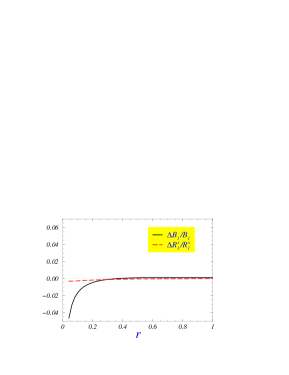
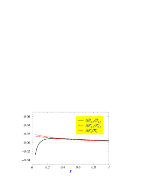
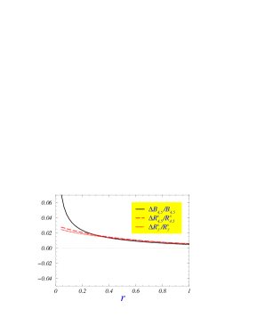
Figure 1: Finite volume effects for the $B_{1-5}$-parameters, computed by using eq. (4.1), are denoted by the thick solid curves, whereas those corresponding to the silver combinations $R_{1-7}^{s}$ are represented by the dashed and dotted thick lines. The plots are made for $L=2\,{\rm fm}$. Notice that $r=m_{u/d}/m_{s}$ is varied by keeping $m_{s}$ fixed to its physical value. To better appreciate the benefit of using $R_{1-7}^{s}$ we also show the line corresponding to zero finite volume effect (thin dashed line).

We first observe the usual behavior, namely that the finite volume effects become larger as one is getting closer to the physical point, i.e., $r=0.04$ [14]. Secondly, we see that the finite volume effects on the silver combinations, $R_{1-7}^{s}$, are clearly reduced when confronted to those that plague $B_{1-5}$-parameters. Finally, we stress again that the leading finite volume effects on the golden ratios [eq. (15)] are totally absent.

5 $K\to\pi$ case

The discussion of the previous section can be easily extended to the $K\to\pi$ case which is often considered on the lattice when computing the $\Delta I=3/2$ amplitude in $K\to\pi\pi$ decay. A golden log-free combination can be easily constructed from the chiral logarithmic corrections to the electro-weak penguin operators calculated in, for example, ref. [15].

To be more specific we will concentrate on the following three operators:

$$Q_{7}^{3/2} = \bar{s}\gamma_{\mu}^{L}u\,\bar{u}\gamma_{\mu}^{R}d+\bar{s}\gamma_{\mu}^{L}d\,(\bar{u}\gamma_{\mu}^{R}u-\bar{d}\gamma_{\mu}^{R}d),$$

$$Q_{8}^{3/2} = \bar{s}^{i}\gamma_{\mu}^{L}u^{j}\,\bar{u}^{j}\gamma_{\mu}^{R}d^{i}+\bar{s}^{i}\gamma_{\mu}^{L}d^{j}\,(\bar{u}^{j}\gamma_{\mu}^{R}u^{i}-\bar{d}^{j}\gamma_{\mu}^{R}d^{i}),$$ (22)

$$Q_{27}^{3/2}\equiv Q_{9}^{3/2} = \bar{s}\gamma_{\mu}^{L}u\,\bar{u}\gamma_{\mu}^{L}d+\bar{s}\gamma_{\mu}^{L}d\,(\bar{u}\gamma_{\mu}^{L}u-\bar{d}\gamma_{\mu}^{L}d),$$

where $\gamma_{\mu}^{R/L}=\gamma_{\mu}(1\pm\gamma_{5})$. The chiral representation of these operators reads

$$Q_{7}^{3/2} = -b_{2}{f^{4}\over 4}B_{0}^{2}\left(\Sigma^{\dagger}_{du}\Sigma_{us}-\Sigma^{\dagger}_{dd}\Sigma_{ds}+\Sigma^{\dagger}_{uu}\Sigma_{ds}\right),$$

$$Q_{8}^{3/2} = -b_{3}{f^{4}\over 4}B_{0}^{2}\left(\Sigma^{\dagger}_{du}\Sigma_{us}-\Sigma^{\dagger}_{dd}\Sigma_{ds}+\Sigma^{\dagger}_{uu}\Sigma_{ds}\right),$$ (23)

$$Q_{27}^{3/2} = -b_{1}{f^{4}\over 8}\left\{(\Sigma^{\dagger}\partial_{\mu}\Sigma)_{ds}[(\Sigma^{\dagger}\partial_{\mu}\Sigma)_{uu}-(\Sigma^{\dagger}\partial_{\mu}\Sigma)_{dd}]+(\Sigma^{\dagger}\partial_{\mu}\Sigma)_{us}(\Sigma^{\dagger}\partial_{\mu}\Sigma)_{du}\right\}.$$

The relevant matrix elements are parameterized as

$$\langle\pi^{+}|Q_{7}^{3/2}|K^{+}\rangle = -{2\over 3}\,\left({m_{K}\over m_{s}+m_{d}}\right)^{2}m_{K}^{2}f_{K}^{2}B_{5}^{K\pi},$$

$$\langle\pi^{+}|Q_{8}^{3/2}|K^{+}\rangle = -2\,\left({m_{K}\over m_{s}+m_{d}}\right)^{2}m_{K}^{2}f_{K}^{2}B_{4}^{K\pi},$$ (24)

$$\langle\pi^{+}|Q_{27}^{3/2}|K^{+}\rangle = {4\over 3}\ m_{K}m_{\pi}f_{K}^{2}B_{1}^{K\pi},$$

where the bag parameters $B_{1,4,5}^{K\pi}$ are the $K\to\pi$ versions of the $K^{0}\!-\!{\overline{K^{0}}}$ ones, discussed in the previous section. They both have the same tree level values but differ in the chiral logarithmic corrections, which we computed as well and obtained

$$B_{1}^{K\pi} = B_{1}^{\rm tree}\left[1-\frac{1}{4(4\pi f)^{2}}\,\left(\frac{5m_{K}-13m_{\pi}}{m_{K}-m_{\pi}}m_{\pi}^{2}\log\frac{m_{\pi}^{2}}{\mu^{2}}+2\frac{3m_{K}+m_{\pi}}{m_{K}-m_{\pi}}m_{K}^{2}\log\frac{m_{K}^{2}}{\mu^{2}}\right.\right.$$

$$\left.\left.\hskip 223.35413pt-3m_{\eta}^{2}\log\frac{m_{\eta}^{2}}{\mu^{2}}\right)+\dots\right],$$

$$B_{4}^{K\pi} = B_{4}^{\rm tree}\left[1+\frac{1}{4(4\pi f)^{2}}\,\left(\frac{3m_{K}+5m_{\pi}}{m_{K}-m_{\pi}}m_{\pi}^{2}\log\frac{m_{\pi}^{2}}{\mu^{2}}+2\frac{m_{K}-5m_{\pi}}{m_{K}-m_{\pi}}m_{K}^{2}\log\frac{m_{K}^{2}}{\mu^{2}}\right.\right.$$ (25)

$$\left.\left.\hskip 223.35413pt-\frac{7}{3}m_{\eta}^{2}\log\frac{m_{\eta}^{2}}{\mu^{2}}\right)+\dots\right],$$

$$B_{5}^{K\pi} = B_{5}^{\rm tree}\left[1+\frac{1}{4(4\pi f)^{2}}\,\left(\frac{3m_{K}+5m_{\pi}}{m_{K}-m_{\pi}}m_{\pi}^{2}\log\frac{m_{\pi}^{2}}{\mu^{2}}+2\frac{m_{K}-5m_{\pi}}{m_{K}-m_{\pi}}m_{K}^{2}\log\frac{m_{K}^{2}}{\mu^{2}}\right.\right.$$

$$\left.\left.\hskip 223.35413pt-\frac{7}{3}m_{\eta}^{2}\log\frac{m_{\eta}^{2}}{\mu^{2}}\right)+\dots\right].$$

Therefore, the chiral extrapolation of the ratio of matrix elements of the electro-weak penguin operators, i.e.,

$$R_{2}^{g\ K\pi}={B_{4}^{K\pi}\over B_{5}^{K\pi}}\,,$$ (26)

that can be computed on the lattice, is free from uncertainties induced by the inclusion of the chiral logarithms in chiral extrapolations. In addition, the leading finite volume effects in the ratio $R_{2}^{g\ K\pi}$ completely cancel. The absolute values for $B_{1,4,5}^{K\pi}$, on the other hand, can be extracted from the following silver relations:

$$R^{s\ K\pi}_{1}=\frac{f_{K}}{f_{\pi}}B_{1}^{K\pi}\,,\qquad R^{s\ K\pi}_{4,5}={f_{K}}\,B_{4,5}^{K\pi}\,.$$ (27)

We believe the safe extrapolation of the lattice results for $R_{2}^{g\ K\pi}$ may be useful in disentangling the current discrepancies among various analytic [16] and lattice approaches [17] used so far to estimate $\langle\pi^{+}|Q_{8}^{3/2}|K^{+}\rangle$. Even more so after noticing that almost all approaches agree in the value for $B_{5}^{K\pi}$, while they differ quite a lot in that for $B_{4}^{K\pi}$. Finally, a reader interested in the discussion of the potential SUSY enhancement of the $\Delta I=3/2$ amplitude is referred to ref. [18].

6 Golden ratios and next-to–next-to leading (NNLO) chiral corrections

We showed that the golden ratios were completely protected against the presence of the chiral logarithms and thus also against the finite volume corrections. One may wonder if that feature survives after accounting for higher order corrections in the chiral expansion. That question was recently rised in ref. [19] where it has been argued that the pion mass might receive sizable finite volume NNLO chiral corrections. That issue will obviously be settled only after the full $2$-loop chiral corrections in finite volume are computed. Here we discuss such corrections to our golden ratios $R_{1,2}^{g}$, and argue that in this case the finite volume corrections arising beyond $1$-loop ChPT are indeed negligible. Golden ratios are generically defined as

$$R^{g}={\langle out|{\cal O}_{A}|in\rangle\over\langle out|{\cal O}_{B}|in\rangle}\,,$$ (28)

where ${\cal O}_{A}$ and ${\cal O}_{B}$ are two different operators with the same chiral representation. The NNLO chiral expansion to this ratio can be schematically written as

$$R^{g} = \frac{g_{A}[1+(logs+c_{A})+(dlogs+clogs_{A}+C_{A})+\dots]}{g_{B}[1+(logs+c_{B})+(dlogs+clogs_{B}+C_{B})+\dots]}$$

$$= \frac{g_{A}}{g_{B}}\biggl{\{}1+(c_{A}-c_{B})+\left[(clogs_{A}-clogs_{B})+(c_{B}-c_{A})(c_{B}+logs)+(C_{A}-C_{B})\right]+\dots\biggr{\}},$$

where $g_{A}/g_{B}$ is the tree level value of the golden ratio, $c_{A,B}$ and $C_{A,B}$ are the low energy constants arising at NLO and NNLO respectively, $clogs_{A,B}$ are the $1$-loop part to the NNLO correction. Based on the same argument used in sec. 3, the single and double chiral logarithms, $logs$ and $dlogs$, completely cancel in the ratio and thus the computation of the NNLO chiral corrections comprises the $1$-loop diagrams only. That feature clearly holds at any other higher order, i.e. one needs to compute the diagrams that are one loop less with respect to the ones indicated by the canonical ChPT counting.

After including the NNLO corrections, the finite volume effects to the golden ratio can be written in the following form:

$${\Delta R^{g}\over R^{g}}\equiv{R^{gL}-R^{g\infty}\over R^{g\infty}}=\Delta clogs_{A}-\Delta clogs_{B}+(c_{B}-c_{A})\Delta logs\,,$$ (30)

in an obvious notation. We see that the finite volume effects arise only from the $1$-loop diagrams at the weak vertices, and therefore the result can be expressed in terms of the $\xi_{s}$-function, as before.

To exemplify the above discussion we now use the set of counterterm lagrangians, written explicitely in ref. [20], to obtain the counterterm contributions to the NLO expression for $R_{2}^{g}$. Those are then used to calculate the finite volume corrections to $R_{2}^{g}$ at NNLO. We obtain 

$${\Delta R^{g}_{2}\over R^{g}_{2}} = -\frac{1}{12\,f^{2}}\left\{12\,m_{K}^{2}\,\left[{{\delta}_{1}}+3\,{{\delta}_{2}}+2\,\left(-3\,{{\delta}_{3}}+8\,{{\delta}_{4}}+8\,{{\delta}_{5}}+8\,{{\delta}_{6}}-4\,{{\delta}_{7}}\right)\right]\,\xi_{\frac{1}{2}}(L,{m_{K}})\right.$$ (31)

$$+3\,\left[8\,m_{K}^{2}\,{{\delta}_{2}}-{{m_{\pi}}}^{2}\,\left({{\delta}_{1}}+{{\delta}_{2}}+4\,\left(3\,{{\delta}_{3}}-5\,{{\delta}_{4}}-5\,{{\delta}_{5}}-6\,{{\delta}_{6}}+6\,{{\delta}_{7}}\right)\right)\right]\,\xi_{\frac{1}{2}}(L,{m_{\pi}})$$

$$+\,\left[32\,m_{K}^{2}\,\left({{\delta}_{4}}+{{\delta}_{5}}+{{\delta}_{6}}\right)-4m_{\pi}^{2}\,\left(3\,{{\delta}_{4}}+3\,{{\delta}_{5}}+2\,{{\delta}_{6}}\right)\right.$$

$$\qquad\left.\left.-m_{\eta}^{2}\,\left({{\delta}_{1}}+17\,{{\delta}_{2}}+20\,{{\delta}_{3}}+24\,{{\delta}_{7}}\right)\right]\,\xi_{\frac{1}{2}}(L,{m_{\eta}})\right\}.$$

Notice that the double pole contributions ($\propto\xi_{\frac{3}{2}}$) coming from NLO² and from NNLO terms, cancel against each other. The size of the finite volume corrections evidently depends on the values for the low energy constant $\delta_{i}$. By using either the naïve dimensional analysis or the values extracted from the recent quenched lattice data , we get that for $L\geq 1.5$ fm and $r\in[0.04,1)$, the finite volume effects, $\Delta R^{g}_{2}/R^{g}_{2}$, are within a few per mil, thus totally negligible.

7 Summary

In this work we computed the $1$-loop chiral corrections to the bag parameters that are relevant to the $K^{0}\!-\!{\overline{K^{0}}}$ mixing amplitude in the SUSY extensions of the SM. Two out of five independent $\Delta S=2$ operators have reversed color indices so that their chiral log corrections are identical to those in which the color indices are not reversed. This “color blindness”, which also emerges from the explicit calculation in the chiral representation of those $\Delta S=2$ operators, is actually expected since the change of the color structure of the operators is a local effect which cannot appear in chiral loops. Rather it is encoded in the low energy constants. After comparing the $1$-loop chiral expressions for all the bag parameters obtained in finite and infinite volume, we also provide the formulae for the finite volume effects which are useful for the assessment of the associated systematic uncertainty in the lattice calculations. As in our previous paper [10], we see that the finite volume effects become more pronounced as the light valence quark of the neutral kaon gets closer to the chiral limit. We find that the combinations of bag parameters in which the chiral logarithmic dependence cancels partly or totally may be particularly beneficiary for the lattice calculations because they allow one to sensibly reduce two important sources of systematic uncertainties: (i) the errors induced by the chiral extrapolations, and (ii) the errors due to the finiteness of the lattice box. We construct the explicit combinations of bag parameters that are log-safe, i.e., in which the chiral logarithms cancel either totally (golden combinations, $R^{g}_{1,2}$) or partially (silver combinations, $R^{s}_{1-7}$). In addition, we show that inclusion of the NNLO corrections does not spoil the advanteges of computing the golden ratio on the lattice. A similar discussion is also made for the case of the $K\to\pi$ matrix elements of the electro-weak penguin operators.

References

• [1] D. Becirevic, Nucl. Phys. Proc. Suppl.  129-130 (2004) 34.
• [2] M. Battaglia et al., hep-ph/0304132; J. Charles et al. [CKM fitter Group Collaboration], hep-ph/0406184.
• [3] A. D. Sakharov, Pisma Zh. Eksp. Teor. Fiz.  5 (1967) 32 [JETP Lett.  5 (1967 SOPUA,34,392-393.1991 UFNAA,161,61-64.1991) 24].
• [4] L. J. Hall, V. A. Kostelecky and S. Raby, Nucl. Phys. B 267 (1986) 415.
• [5] C. R. Allton et al., Phys. Lett. B 453 (1999) 30 [hep-lat/9806016]; D. Becirevic et al., Nucl. Phys. Proc. Suppl.  106 (2002) 326 [hep-lat/0110006].
• [6] M. Ciuchini et al., JHEP 9810 (1998) 008 [hep-ph/9808328]; D. A. Demir, A. Masiero and O. Vives, Phys. Rev. Lett.  82 (1999) 2447 [hep-ph/9812337]; S. Baek, J. H. Jang, P. Ko and J. H. Park, Nucl. Phys. B 609 (2001) 442 [hep-ph/0105028]; S. Khalil and O. Lebedev, Phys. Lett. B 515 (2001) 387 [hep-ph/0106023]; A. J. Buras, P. H. Chankowski, J. Rosiek and L. Slawianowska, Nucl. Phys. B 619 (2001) 434 [hep-ph/0107048]; M. Frank and S. Q. Nie, Phys. Rev. D 67 (2003) 115008 [hep-ph/0303115].
• [7] F. Gabbiani, E. Gabrielli, A. Masiero and L. Silvestrini, Nucl. Phys. B 477 (1996) 321 [hep-ph/9604387].
• [8] M. Ciuchini et al., Nucl. Phys. B 523 (1998) 501 [hep-ph/9711402]; A. J. Buras, M. Misiak and J. Urban, Nucl. Phys. B 586 (2000) 397 [hep-ph/0005183].
• [9] R. Gupta, T. Bhattacharya and S. R. Sharpe, Phys. Rev. D 55 (1997) 4036 [hep-lat/9611023].
• [10] D. Becirevic and G. Villadoro, Phys. Rev. D 69 (2004) 054010 [hep-lat/0311028].
• [11] J. F. Donoghue, E. Golowich and B. R. Holstein, “Dynamics Of The Standard Model”, Cambridge Monogr. Part. Phys. Nucl. Phys. Cosmol.  2 (1992) 1; H. Leutwyler, “Chiral dynamics”, hep-ph/0008124; A. Pich, Rep. Prog. Phys.  58 (1995) 563 [hep-ph/9502366]; G. Ecker, “Strong interactions of light flavours”, hep-ph/0011026; U. G. Meissner, Rep. Prog. Phys.  56 (1993) 903 [hep-ph/9302247]; G. Colangelo, G. Isidori, “An introduction to ChPT”, hep-ph/0101264.
• [12] J. Gasser and H. Leutwyler, Nucl. Phys. B 250 (1985) 465.
• [13] J. Gasser and H. Leutwyler, Phys. Lett. B 184 (1987) 83.
• [14] H. Leutwyler, Phys. Lett. B 378 (1996) 313 [hep-ph/9602366].
• [15] V. Cirigliano and E. Golowich, Phys. Rev. D 65 (2002) 054014 [hep-ph/0109265].
• [16] M. Knecht, S. Peris and E. de Rafael, Phys. Lett. B 508 (2001) 117 [hep-ph/0102017]; E. Pallante, A. Pich and I. Scimemi, Nucl. Phys. B 617 (2001) 441 [hep-ph/0105011]; J. Bijnens, E. Gamiz and J. Prades, JHEP 0110 (2001) 009 [hep-ph/0108240]; V. Cirigliano, J. F. Donoghue, E. Golowich and K. Maltman, Phys. Lett. B 555 (2003) 71 [hep-ph/0211420]; S. Bertolini, J. O. Eeg and M. Fabbrichesi, Phys. Rev. D 63 (2001) 056009 [hep-ph/0002234]; S. Narison, Nucl. Phys. B 593 (2001) 3 [hep-ph/0004247].
• [17] A. Donini, V. Gimenez, L. Giusti and G. Martinelli, Phys. Lett. B 470 (1999) 233 [hep-lat/9910017]; J. I. Noaki et al. [CP-PACS Collaboration], Phys. Rev. D 68 (2003) 014501 [hep-lat/0108013]; T. Blum et al. [RBC Collaboration], Phys. Rev. D 68 (2003) 114506 [hep-lat/0110075].
• [18] A. L. Kagan and M. Neubert, Phys. Rev. Lett.  83 (1999) 4929 [hep-ph/9908404].
• [19] G. Colangelo and S. Durr, Eur. Phys. J. C 33 (2004) 543 [hep-lat/0311023].
• [20] V. Cirigliano and E. Golowich, Phys. Lett. B 475 (2000) 351 [hep-ph/9912513].