Electric Polarizability of Neutral Hadrons from Lattice QCD

Abstract

By simulating a uniform electric field on a lattice and measuring the change in the rest mass, we calculate the electric polarizability of neutral mesons and baryons using the methods of quenched lattice QCD. Specifically, we measure the electric polarizability coefficient from the quadratic response to the electric field for 10 particles: the vector mesons $\rho^{0}$ and $K^{*0}$; the octet baryons n, $\Sigma^{0}$, $\Lambda_{o}^{0}$, $\Lambda_{s}^{0}$, and $\Xi^{0}$; and the decouplet baryons $\Delta^{0}$, $\Sigma^{*0}$, and $\Xi^{*0}$. Independent calculations using two fermion actions were done for consistency and comparison purposes. One calculation uses Wilson fermions with a lattice spacing of $a=0.10\,$fm. The other uses tadpole improved Lüsher-Weiss gauge fields and clover quark action with a lattice spacing $a=0.17\,$fm. Our results for neutron electric polarizability are compared to experiment.

I Introduction and Review

Electric and magnetic polarizabilities characterize the rigidity of both charged and uncharged hadrons in external fields and are important fundamental properties of particles. In particular, the electric polarizability of a hadron characterizes the reaction of quarks to a weak external electric field and can be measured by experiment via Compton scattering. In this paper we describe a lattice quantum chromodynamics (QCD) calculation of neutral hadron electric polarizabilities using an external field method. The goal of Monte Carlo lattice QCD is to extract fundamental, measurable quantities directly from the theory without model assumptions. Learning about such aspects of particles tests our understanding and formulation of the underlying theory and makes new aspects and predictions of the theory subject to experimental verification. Such calculations can give insights on the internal structure of hadrons and the applicability of chiral perturbation theory to various low energy aspects of lattice QCD.

Conceptually, electric and magnetic fields, even from a single photon, will distort the shape of a hadron, thereby affecting the internal energy and thus the mass. The electric and magnetic polarizabilities are defined as the coefficients of the quadratic electric and magnetic field terms in the mass shift formula ($\hbar=c=1$ gaussian units):

$$\Delta m=-\frac{1}{2}\,\alpha\vec{E}^{2}-\frac{1}{2}\,\beta\vec{B}^{2},$$ (1)

where ${\alpha}$ $(\beta)$ is the electric (magnetic) polarizability that compares to experiment. When the terms in Eq.(1) are viewed as the non-relativistic interaction Hamiltonian, one obtains the polarized on-shell Compton scattering cross section for neutral particles:

$$\frac{d\sigma}{d\Omega}=\frac{1}{(4\pi)^{2}}\left(\frac{\omega_{2}}{\omega_{1}}\right)|\,\alpha\,\omega_{1}\,\omega_{2}\,(\hat{\epsilon_{1}}\cdot\hat{\epsilon_{2}}^{*})+\beta\,(\hat{\epsilon_{1}}\times\vec{k}_{1})\cdot(\hat{\epsilon_{2}}^{*}\times\vec{k}_{2})\,|^{2}.$$ (2)

$\omega_{1,2}$ and $\vec{k}_{1,2}$ are the initial, final photon angular frequencies and wave vectors and $\hat{\epsilon}_{1,2}$ are the polarization vectors. (The quantity $\omega_{2}/\omega_{1}$ is a recoil factor and can be ignored nonrelativistically.) This allows hadron polarizabilities to be measured in scattering experiments. (For charged spinless particles one must also add the Thompson scattering amplitude from the particle’s charge and, if virtual, a charge radius term before calculating the cross section. See Eq.(11) of wil1 .) Compilations of experimental results for neutron electric polarizability have been given in chr1 ; Zhou:2004 . Although the polarizabilities of the other particles investigated here have not been measured, we hope that the comparison of the results from the various types of mesons and baryons investigated will give insights on their relative rigidity and structure.

The lattice calculation of electric polarizabilities began with the paper by Fiebig et al. Fiebig:1989en using the staggered fermion formulation of lattice quarks. An external electric field was simulated on the lattice and mass shifts measured directly for the neutron and neutral pion. Although the simulation errors were large, the neutron electric polarizability extracted there is now seen to be in remarkable agreement with recent experiments. Lattice four point function techniques have also been designed to extract neutral or charged particle electric polarizabilities wil1 (chiral symmetry can sometimes be used to reduce the calculation to two point functions wil2 ), but these methods are more difficult to carry out on the lattice. Early results of the present study have been reported in chr1 . See Zhou:2002 for preliminary results of a companion calculation of the magnetic polarizability of both charged and uncharged hadrons.

II Lattice Details

The clover part lush of this calculation uses the tadpole-improved clover action with coupling constant $c_{SW}=1/u_{0}^{4}$, where $u_{0}^{4}$ is the average plaquette. We use the zero-loop, tadpole improved Lüsher-Weiss gauge field action on a quenched $12^{3}\times 24$ lattice with $\beta=7.26$ ($a_{\rm clover}=0.17\,{\rm fm}$). In both Wilson and clover cases the gauge field was thermalized by 10,000 sweeps (quasi-heatbath with overrelaxation) and then saved every 1000. We have used 100 configurations in the clover case. In the Wilson case the lattice is $24^{4}$ and we used 109 configurations with standard gauge field action with $\beta=6.0$ ($a_{\rm Wilson}=0.1\,{\rm fm}$) gock . Our quark propagator time origin, $t=0$, was chosen to be the third lattice time step for clover fermions and the second time step in the Wilson case. Point quark sources were constructed for the zero momentum quark propagators. The standard particle interpolation fields for the octet terry1 (non-relativistically non-vanishing) and decouplet terry2 baryons were used. Periodic boundary conditions in the spatial directions and free or Dirichlet boundary conditions for the time links on the lattice time edges were used.

As is usual in lattice calculations, the mass of a hadron can be calculated from the exponential time decay of a correlation function. By calculating the ratio of the correlation function in the field to that without the field, we have a ratio of exponentials which decays at the rate of the mass difference. According to Eq.(1), the electric mass shifts should be parabolic, negative mass shifts giving positive polarizability coefficients and positive shifts giving negative coefficients. We use four values of the electric field to establish the parabola. Following the technique in Fiebig:1989en , we will average the correlation functions over $\vec{E}$ and $-\vec{E}$ in order to remove the spurious linear term in the parabolic fits. We include the uniform static E-field as a phase on the gauge links in a particular direction (with fermion charge $q=Qe$):

$$e^{iaqA}=e^{i(a^{2}qE)(x_{4}/a)}=e^{i\eta\tau}\rightarrow(1+i\eta\tau).$$ (3)

There is a discontinuity in the electric field at the decoupled lattice time boundary under this formulation, which should not be a problem as all of our correlation functions are measured far from the time edges of our lattices. Since the electric field is linearized in the continuum, we used the linearized form on the lattice. Fiebig et al. found no significant difference between the exponential and linearized formats for similar electric fields.

On the lattice we have an exact SU(2) isospin symmetry. This symmetry is broken by the different electric charges on the u- and d-quarks in the presence of the external electric field. Consequently the $\pi^{0}$ and $\rho^{0}$ $I=$1 particles can mix with $I=0$ glueballs and disconnected quark loops (self-contractions of the interpolation fields) can propagate these particles. Disconnected loop methods have been considerably improved in recent years defl ; however, calculation of these diagrams is still extremely time consuming. In this paper, we will ignore the effect of the disconnected loops.

Including the static electric field as a phase on the links affects the Wilson term, but not the clover loops. This is clear since the conserved vector current derived by the Noether procedure is identical for the clover and Wilson actions. In units of $10^{-3}e^{-1}a^{-2}$, the electric field took the values $\pm 1.08$, $\pm 2.16$, $\pm 4.32$, and $\pm 8.64$ via the parameter $\eta=a^{2}QeE$ in Eq. (3) for both the clover and Wilson cases. (The $\eta$ values were $\pm 0.00036,\pm 0.00072,\pm 0.00144,\pm 0.00288$, and $\pm 0.00576$, the same as in Ref. Fiebig:1989en .) In conventional units the smallest electric field is approximately $7.4\times 10^{21}$ N/C in the clover case [$(.17/.1)^{2}=2.35$ times larger in the Wilson case], which is about the same electric field strength $.26\,{\rm fm}$ from a d-quark. Although these are huge fields, we will nevertheless see that the lattice mass shifts are small and that there is no evidence of $E^{4}$ or higher terms in the electric field fits. We will in fact check that a drastic reduction in the field does not change the polarizability coefficients.

We did the calculation with both Wilson and clover fermions in order to test the consistency of our results as well as to set benchmarks for future polarizability calculations. We do not expect that the two formulations will agree with one another throughout the mass range investigated. As in any lattice calculation, there are many sources of systematic error, including quenching, finite volume, and finite size errors. The finite volume errors for the Wilson case ($L\simeq 2.4$ fm) should be slightly smaller than for clover ($L\simeq 2$ fm); however, discretization errors should be smaller for the clover case. In addition, to achieve physical results, a chiral extrapolation to physical quark masses is necessary. The quenched chiral regime has been estimated to extend to pion masses of only about $300$ MeV kehfei for the pseudoscalar decay constant, $f_{P}$, and the ratio $m_{\pi}^{2}/m$, where $m$ is the quark mass, although this does not exclude the range being larger for other quantities. Our pion masses are almost certainly too large to get into the chiral regime and we do not attempt a chiral extrapolation here. However, we would expect the agreement between the two calculations to improve at our lower pion masses, which is what is seen. Our pion masses here range from about 1 GeV to about 500 MeV; we achieve the smallest pion mass in the case of clover fermions, 483 MeV.

With $\kappa_{\rm cr}=0.1232(1)$ in the clover case, we used six values of $\kappa=0.1182$, $0.1194$, $0.1201$, $0.1209$, $0.1214$, and $0.1219$, which roughly correspond to $m_{q}\sim 200$, $150$, $120$, $90$, $70$, and $50$ MeV. The critical value of $\kappa$ for the Wilson case is $0.157096(28)^{+33}_{-9}$ iwasaki . The values of $\kappa$ used in the Wilson calculation were $0.1515,0.1525,0.1535,0.1540,0.15454$, and $0.1555$, which correspond to approximate quark masses of $m_{q}\sim 232$, $189$, $147$, $126$, $106$, and $65$ MeV. We choose $\kappa=0.1201$ to represent clover strange quarks and $\kappa=0.1540$ to represent Wilson strange quarks. We used multi-mass BiCGStab as the inversion algorithm for both the clover and Wilson cases. The number of quark inversions per gauge field and quark mass was 11: 10 values of $\eta$ in Eq.(3) associated with 4 nonzero electric fields for both the u and d-quarks, plus the zero field inversion. Our Wilson and clover calculations were done completely independently from one another.

III Results

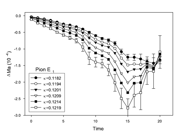
Figure 1: The effective lattice mass shift, $\Delta Ma$, for the $\pi^{0}$ for the six quark masses in the clover study for the smallest electric field value. Error bars are shown only on the $\kappa=0.1182,0.1219$ values.

Figure 2: The effective lattice mass shift, $\Delta Ma$, for the $\pi^{0}$ for the six quark masses in the Wilson study for the smallest electric field value. Error bars are shown only on the $\kappa=0.1515,0.1555$ values.

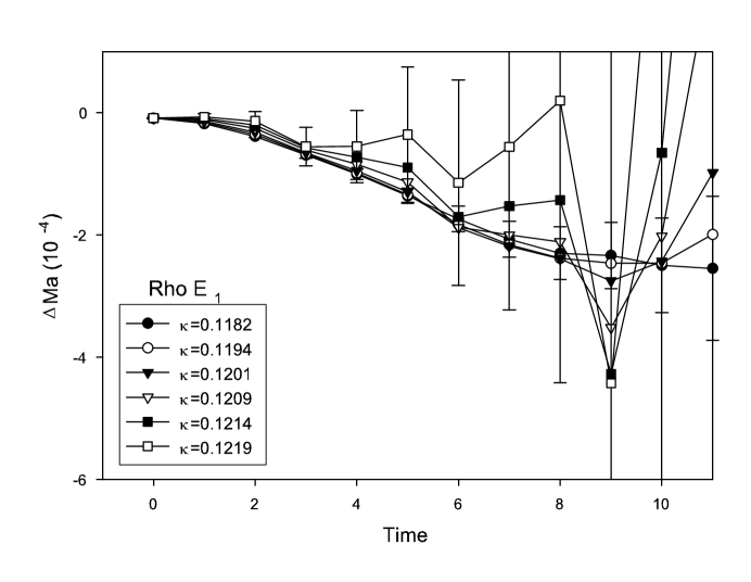
Figure 3: Same as Fig. 1 (clover case) except for the $\rho^{0}$.

Figure 4: Same as Fig. 2 (Wilson case) except for the $\rho^{0}$.

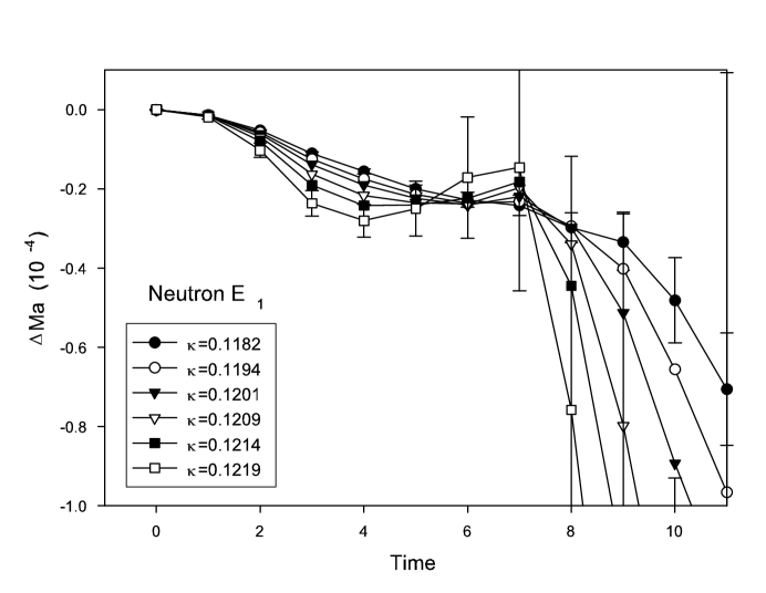
Figure 5: Same as Fig. 1 (clover case) except for the neutron.

Figure 6: Same as Fig. 2 (Wilson case) except for the neutron.

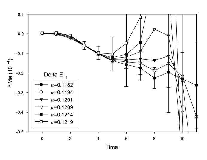
Figure 7: Same as Fig. 1 (clover case) except for the $\Delta^{0}$.

Figure 8: Same as Fig. 2 (Wilson case) except for the $\Delta^{0}$.

We start with an examination of the effective mass shifts of the four non-strange particles in this study, $\pi^{0}$, $\rho^{0}$, neutron, and $\Delta^{0}$, as a function of lattice time; see Figs. 2-8. The effective mass shift for each particle is defined to be

$$R(t)=\frac{G_{E}(t)}{G_{0}(t)},$$ (4)

$$\Delta Ma\,(t)\equiv\ln\,(\frac{R(t)}{R(t+1)}).$$ (5)

where $G_{0}(t)$ is the particle propagator without an electric field and $G_{E}(t)$ is the value with the field. The notation $\Delta Ma\,(t)$ indicates this value is being associated with the time point $t$ (measured from the hadron source) in the graphs. These figures are used to guide us in the choice of optimal propagator time points in the fits. Just as single exponential behavior should emerge for each particle channel in Euclidean time, the ratio of particle propagators must also become single exponential. This means, from Eq.(5), that the effective mass shift plot should become time independent. As in most lattice simulations, particle propagators become increasing noisy as lattice time increases, so the mass shift data will eventually become dominated by statistical errors at large time separations. We will examine the results at the lowest electric field value; the effective mass shifts at larger fields we will soon see is simply scaled with the $E^{2}$ value.

Figs. 2, 4, 6, and 8 give the non-strange hadron mass shifts for six quark masses of clover fermions; Figs. 2, 4, 6, and 8 give similar shifts for six Wilson masses. Error bars computed with the jackknife technique are shown on the largest and smallest quark mass results to give an idea of the statistical errors. We show only those lattice time points which we feel have meaningful Monte Carlo values in each of these graphs for clarity. Our pion result, Figs. 2 and 2, is surprising. We never do see the expected time independence of the mass shift for any value of the quark mass. Our results in Figs. 2 and 2 are plotted out to the final time step (20 in the clover case, 21 in the Wilson) to show the complete time history. There is apparently a dip in the time behavior for clover fermions near $t=15$, but our error bars are too large at this point to confirm this as a plateau. The Wilson case also has no convincing plateau. We note that Fiebig et al. Fiebig:1989en isolated a small signal for the neutral pion in their calculations. They used staggered fermions, which have a reminant exact chiral symmetry. Of course the chiral symmetry is broken for both Wilson and clover fermions, and this could be the crucial difference in the calculations. It is possible that the neglect of the disconnected diagrams could be responsible for the bad pion behavior. The prediction from chiral perturbation theory is that $\alpha_{\pi^{0}}$ should be small and negative: $\alpha_{\pi^{0}}=-0.35\pm.1\times 10^{-4}$ fm³ bell .

The other particle channels studied behave conventionally. Figs. 4 and 4 show the time evolution of the $\rho^{0}$ signal, which is very noisy. Although the signal decays quickly, a short time plateau is apparent in the data for both clover and Wilson fermions. Similar behavior is seen in Figs. 6 and 6 in the case of the neutron, for which the statistical signal is better. (Fig. 9 shows the clover neutron mass shifts out to $t=16$, and will be discussed below.) A plateau also appears in Figs. 8 and 8 for the $\Delta^{0}$. The time plateaus appear at larger time steps for the Wilson data, as would be expected from the smaller value of the lattice spacing. The optimal time fit ranges are a compromise between statistical errors and systematic time evolution. Using the effective mass shift results and chi-square values as a guide, and assuming single exponential time fits of the ratio, $R(t)$, we fit propagator ratio data for a given particle, mass, and electric field across three time steps. Although we find that it is often possible to fit at smaller times for larger $\kappa$, we prefer to choose time plateau ranges independent of the quark mass being studied in order to avoid introducing spurious systematic effects.

For clover data, a time plateau in the mass shift data for the neutron, Fig. 6, begins about time step $5$. We take this as typical of the octet baryons and fit the others in this same time range. The $\Delta^{0}$ in Fig. 8 is noisier than the neutron but also has a plateau in the same region, evident for the heavier masses; we fit the same time range for the decouplets as for the octets. The $\rho^{0}$ in Fig. 4 is even noisier than the $\Delta^{0}$, but has a plateau with acceptable chi-square values slightly further from the time origin. Our final choices for the optimal time plateaus are $t=5-7$ for the octets and decouplet particles, and $t=6-8$ for the $\rho^{0}$ and $K^{*0}$. Similar considerations guide our choices of time plateaus in the Wilson case, and we choose to fit time steps $14-16$ in the case of octet baryons (see Fig. 6) and $9-11$ for the decouplets (Fig. 8), which again are noisier. We also fit the $\rho^{0}$ (Fig. 4) and $K^{*0}$ with time steps $13-15$ and $10-12$, respectively. The $\Lambda^{0}_{s}$, the flavor-singlet octet member, is a special case. It is much noisier than the other octet members and we were not able to extract results from the Wilson simulations with the same time plateau as the other octet baryons. In the clover case, the polarizability is the largest of all the 10 particles listed, but also with very large error bars.

Figs. 9a,b,c, and d are a striking demonstration of the $E^{2}$ dependence of all of our mass shifts. These figures show the mass shifts, Eq.(5), for the neutron for all quark masses and all four nonzero electric field values for clover fermions. Since our nonzero electric field values differ by factors of 2, we have rescaled the mass shifts for each of these by a factor of 4. Clearly, the time evolution of the mass shifts is essentially identical in these graphs - even the error bars scale with the factor of 4. This means that quadratic dependence on the electric field is assured for any choice of time fit range. The other particles, including the pion, display the same type of behavior, and this is seen for both clover and Wilson fermions. When we fit both $E^{2}$ and $E^{4}$ coefficients, we find no evidence of $E^{4}$ or higher terms and the chi-squared values on our electric field parabola fits are quite small.

Although Fig. 9 leaves little doubt about the $E^{2}$ dependence in our electric field range, we decreased the field in the clover calculation by a factor of 10 for the first 20 configurations and reexamined the mass shift plots to see if the parabola shapes changed. The shifts were 100 times smaller than before, but the time behavior of the plots was almost identical to the original field strength configurations for the same 20 configurations.

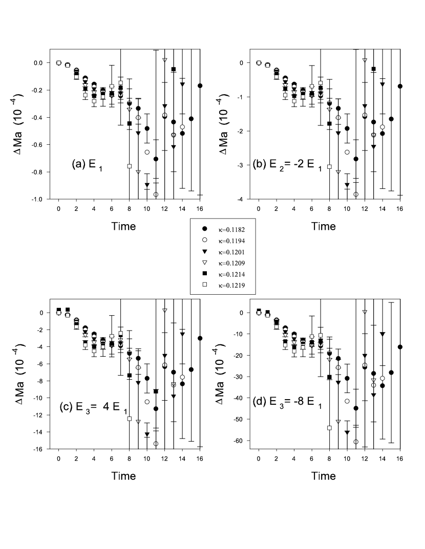
Figure 9: The neutron effective lattice mass shifts, $\Delta Ma$, evaluated for 4 values of the external electric field, E${}_{1}=-1.08\times 10^{-3}e^{-1}a^{-2}$, -2E₁, 4E₁, and -8E₁ in (a)-(d) respectively, for six quark mass values. Error bars shown only on the $\kappa=0.1182,0.1219$ values. The vertical axis scale increases by a factor of 4 in each case, resulting in strikingly similar figures.

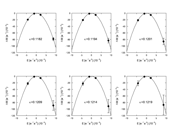
Figure 10: The effective lattice mass shift, $\Delta M$ (in units of $a^{-1}_{\rm clover}$) as a function of electric field in units of $10^{-3}e^{-1}a^{-2}_{\rm clover}$ for the neutron for the six values of quark mass for clover fermions. The time fit range of propagators is 5-7.

Figure 11: The same as Fig. 10, but for Wilson fermions. The time fit range of propagators is 14-16.

Figs. 11 and 11 show examples of fit parabolas and error bars for the neutron for all six values of quark mass. The time fit range of the propagators is $5-7$ in the clover case and $14-16$ in the Wilson case. Again, Fig. 9 guarantees a quadratic field dependence. The averaging procedure described earlier over $\vec{E}$ and $-\vec{E}$ has removed odd terms in the electric field, and we just saw that there is no evidence of $E^{4}$ or higher terms in the results. Figs. 13-20 show the pion mass dependence of the extracted values of the electric polarizability, $\alpha$, for both clover and Wilson fermions. We do not attempt to extract the $\pi^{0}$ or $K^{0}$ polarizabilities because of the problems encountered in finding a fitting plateau. Our clover results for the other non-strange particles are very similar to the preliminary results given in chr1 . We will discuss the particles by groups: first the mesons, next the octet baryons, and finally the decouplet baryons. All are plotted on the same vertical scale ($10^{-4}$ fm³) so that error bars may be compared. Table 1 tabulates the final results for the electric polarizability coefficient for various hadrons for clover fermions; Table 2 gives the same results for the Wilson case.

The results for the $\rho^{0}$ meson are given in Fig. 13. There are definite incompatibilities in the Wilson and clover signals at the larger pion masses. However, as discussed in the last section, we do not necessarily expect the Wilson and clover formulations to agree at the larger pion masses. At the smallest pion masses, the results seem to be becoming more compatible, although the error bars in both cases are getting quite large. The result at our smallest quark mass is in the range $\sim 5-10\times 10^{-4}$ fm³. The results for the $K^{*0}$ are given in Fig. 13. In both calculations there is a significant reduction in the polarizability coefficient for $K^{*0}$ as compared to the $\rho^{0}$; the reduction is slightly larger in the Wilson case. The results for the $K^{*0}$ do not seem to be converging as well as for the $\rho^{0}$ at the smallest quark mass. Note that the fit in the Wilson $K^{*0}$ case has been moved 4 time steps closer to the propagator origin to achieve a signal; this could be contributing to the larger reduction of the Wilson results . The result here is in the range $\sim 1-4\times 10^{-4}$ fm³.

Figure 12: The $\rho^{0}$ meson electric polarizability coefficient, $\alpha$, in units $10^{-4}$ fm³ as a function of the lattice pion mass squared in GeV².

Figure 13: The same as for Fig. 12, except for the $K^{*0}$.

Figure 14: The same as for Fig. 12, except for the neutron. The world average is shown at the physical pion mass squared.

Figure 15: The same as for Fig. 12, except for the $\Sigma^{0}$.

Figure 16: The same as for Fig. 12, except for the $\Lambda^{0}_{o}$.

Figure 17: The same as for Fig. 12, except for the $\Xi^{0}$.

Figure 18: The same as for Fig. 12, except for the $\Delta^{0}$.

Figure 19: The same as for Fig. 12, except for the $\Sigma^{*0}$.

Figure 20: The same as for Fig. 12, except for the $\Xi^{*0}$.

The octet baryons (n, $\Sigma^{0}$, $\Lambda^{0}_{o}$, $\Xi^{0}$) are represented by Figs. 15-17. The signals here are the best of all the particles for both Wilson and clover fermions. The behavior of the all four octet members are quite similar to one another when the Wilson or clover results are compared among themselves. The clover results tend to be a bit larger than the Wilson ones in all cases. All tend to move toward larger values as the pion mass is decreased. There is a convergence of the results for smaller masses. (The $\Xi^{0}$ in Fig. 17 is a possible exception.) As we will discuss shortly, the trend of the neutron results are compatible with experiment. All particles in Figs. 15-17 end up with values in the range of $\sim 10-15\times 10^{-4}$ fm³ at our smallest pion mass. We do not present a graphical result for the $\Lambda^{0}_{s}$, but the values obtained in the clover case are given in Table 1.

The decouplet baryons ($\Delta^{0}$, $\Sigma^{*0}$, $\Xi^{*0}$) are represented by Figs. 19-20. Here the relative signals are not as strong as for the octets (most evident at smaller pion mass) and the values themselves are smaller. Like the octet case, the Wilson or clover decouplet results are quite similar to one another when compared among themselves. While we still have the usual incompatibilities at large pion masses, there is a trend for the results to approach one another for the smaller masses. (The largest disagreement is the $\Xi^{*0}$ in Fig. 20). The results at the smallest pion masses are all on the order of $\sim 2-5\times 10^{-4}$ fm³. This is quite reduced from the octets, whose values range $\sim 10-15\times 10^{-4}$ fm³ for small mass. As in the case of the $K^{*0}$ meson, it was necessary to move the time steps toward the propagator origin in order to achieve a signal in the Wilson case; this could contribute to the relatively large disagreements here between Wilson and clover as opposed to the octet case.

The only experimental result available to us for comparison is the neutron. Because of the absence of free neutron targets, actual Compton scattering experiments must use neutrons bound in the deuteron or other nuclei. The most recent experiments have used either quasi-free deuteron Compton scattering($\gamma\,d\longrightarrow\gamma\,p\,n$) or elastic deuteron scattering ($\gamma\,d\longrightarrow\gamma\,d$). The Particle Data Group result from 2004 for the neutron is $\alpha_{n}=11.6^{+1.9}_{-2.3}$ pdg . The result of a calculation using heavy baryon chiral perturbation theory for the neutron has been given as $13.4\pm 1.5$ BKSM , where the error bars are associated with numerical integration and higher order contributions. Our Wilson and clover results are consistent with these values within Monte Carlo errors at our lowest pion masses, which is very encouraging. However, more work needs to be done, including chiral extrapolations of the present data, before more precise comparisons can be done.

Since the polarizability coefficient scales like length cubed, it is extremely sensitive to the assigned lattice scale, $a$. Clearly, we must get this right if we are to extract experimentally meaningful values for the polarizabilty coefficient. The fact that both our clover and Wilson results for the neutron are tending toward the experimental result at the smallest pion masses is a strong indication of the correctness of our methods. Turning this around, this is a excellent place to set the lattice scale from experiment, once the neutron electric polarizability is determined with greater accuracy.

IV Conclusions

In this study we have used the methods of lattice QCD to evaluate the electric polarizability coefficient for neutral hadrons with both Wilson and clover fermions using improved Lüsher-Weiss gauge fields. We were able to extract and compare electric polarizability coefficients for the vector mesons $\rho^{0}$ and $K^{*0}$; the octet baryons n, $\Sigma^{0}$, $\Lambda_{o}^{0}$, and $\Xi^{0}$; and the decouplet baryons $\Delta^{0}$, $\Sigma^{*0}$, and $\Xi^{*0}$. The $\Lambda_{s}^{0}$ was extracted only in the clover case. As a rule, the Wilson polarizability results are smaller than the clover; however, the two calculations tend to converge at the smallest pion masses studied. We find that the polarizabilities of the octet baryons and of the decouplet baryons behave as a group; all have similar mass dependencies and values when the clover or Wilson results are compared among themselves. This is in stark contrast to the similarity in the charge radii of the proton and charged delta seen in Ref. terry2 . Apparently, the electric polarizability is not correlated to the overall electromagnetic size of the hadron. In addition, Ref. terry2 sees a nontrivial squared charge radius behavior for the neutral baryons, the neutron having a negative charge radius and the others being zero or positive, which also does not seem to be reflected in the polarizability. A simple harmonic oscillator model jackson for charges q and -q in an electric field gives $\alpha=2q^{2}/(m\omega^{2})$ (more generally, one obtains a sum over the squared charges of the constituents), where $m\omega^{2}=k$ is the spring constant. Assuming the constitutent mass, $m$, of the quarks is a constant, a larger energy frequency $\omega$ would explain the smaller polarizability of the decouplets in this model.

The polarizabilities of the octet baryons show the best agreement between clover and Wilson. Outside of the $\Lambda^{0}_{s}$, the polarizabilities mostly tend upward as the pion mass is decreased. They all have values in the neighborhood of $\sim 10-15\times 10^{-4}$ fm³ at the smallest pion mass. Agreement of our results with experiment for the neutron is an encouraging sign. There is more disagreement in the values of the decouplet baryons. Both fermion formulations agree that the values are decreased relative to the octets, but like the $K^{*0}$ relative to the $\rho^{0}$, the reduction is larger for the Wilson case than the clover case. Nevertheless, the clover results are tending downward toward the Wilson values, and both end up with values in the range $2-5\times 10^{-4}$ fm³ at the lowest pion mass. The greatest incompatibility in the calculations appears in the meson sector, especially the $K^{*0}$ vector meson. A possible source of the disagreement between Wilson and clover vector mesons and decouplet baryons seems to be the shorter time interval that was necessary to achieve a signal for these particles in the Wilson case. We have also seen that the pseudoscalar mesons do not have an identifiable mass shift plateau region for either lattice fermion formulation.

Much theoretical work remains to be done in the field of hadron polarizability. Besides extending the present calculations to the chiral regime, magnetic polarizabilities can be measured using external field techniques for both charged and neutral hadrons. Generalized polarizabilities, measured in polarized photon, polarized proton scattering, are beginning to be studied and measured general , and are candidates for lattice calculations. There is also a need to extend chiral perturbation theory calculations of Compton scattering to isolate the polarizability coefficients for mesons and the other octet and decouplet baryons so that chiral extrapolations of lattice data may be done. In addition, the disconnected diagram contribution to the meson polarizabilities and should be investigated, especially in the pseudoscalar channel.

V Acknowledgments

We are grateful to many people and institutions for the resources and time necessary to carry out these investigations. WW would like to thank the Sabbatical Committee of the College of Arts and Sciences of Baylor University as well as the National Science Foundation grant no. 0070836 for support. This work was also partially supported by the National Computational Science Alliance under grants PHY990003N, PHY890044N, PHY040021N and utilized the Origin-2000 and the IBM p690 computers. This author also thanks The George Washington University Physics Department for support through their Center for Nuclear Studies Visiting Scholars Program. In addition, this work has been supported by DOE under grant no. DE-FG02-95ER40907, with computer resources at NERSC and JLAB.

Table 1: The electric polarizabilities from the calculation with clover action using six $\kappa$ values. The units of the electric polarizability are $10^{-4}$ fm³. The pion masses were fit on time steps $11-13$ from the propagator origin and are given in GeV.

$\kappa$	0.1182	0.1194	0.1201	0.1209	0.1214	0.1219
$m_{\pi}$	$0.937\pm.006$	$0.814\pm.007$	$0.735\pm.008$	$0.635\pm.008$	$0.564\pm.009$	$0.483\pm.011$
Mesons							fit range
$\rho^{0}$	11.4 $\pm$ .7	12.0 $\pm$ 1.0	12.2 $\pm$ 1.4	11.8 $\pm$ 2.0	10.7 $\pm$ 3.0	5.9 $\pm$ 5.6	6 to 8
$K^{*0}$	4.7 $\pm$ .4	4.8 $\pm$ .5	4.9 $\pm$ .5	4.8 $\pm$ .7	4.8 $\pm$ .8	4.1 $\pm$ 1.0	6 to 8
Baryon octet
n	12.8 $\pm$ .4	13.6 $\pm$ .6	14.0 $\pm$ .8	14.5 $\pm$ 1.2	14.6 $\pm$ 1.6	14.0 $\pm$ 2.5	5 to 7
$\Sigma^{0}$	11.9 $\pm$ .5	12.0 $\pm$ .7	12.0 $\pm$ .9	11.9 $\pm$ 1.2	11.8 $\pm$ 1.6	11.5 $\pm$ 2.4	5 to 7
$\Lambda^{0}_{o}$	12.5 $\pm$ .4	13.0 $\pm$ .6	13.3 $\pm$ .8	13.6 $\pm$ 1.1	13.9 $\pm$ 1.4	14.1 $\pm$ 1.7	5 to 7
$\Lambda^{0}_{s}$	30 $\pm$ 1	32 $\pm$ 21	40 $\pm$ 24	52 $\pm$ 35	55 $\pm$ 43	53 $\pm$ 86	5 to 7
$\Xi^{0}$	13.4 $\pm$ .5	13.8 $\pm$ .7	14.0 $\pm$ .8	14.2 $\pm$ 1.0	14.5 $\pm$ 1.1	15.1 $\pm$ 1.3	5 to 7
Baryon decuplet
$\Delta^{0}$	8.8 $\pm$ .4	8.4 $\pm$ .6	8.1 $\pm$ .9	7.6 $\pm$ 1.4	6.9 $\pm$ 2.1	5.6 $\pm$ 3.3	5 to 7
$\Sigma^{*0}$	8.0 $\pm$ .4	7.2 $\pm$ .6	6.5 $\pm$ .7	5.5 $\pm$ 1.0	4.5 $\pm$ 1.4	3.5 $\pm$ 2.0	5 to 7
$\Xi^{*0}$	7.3 $\pm$ .5	6.8 $\pm$ .6	6.5 $\pm$ .7	6.1 $\pm$ .9	5.6 $\pm$ 1.2	5.2 $\pm$ 1.5	5 to 7

Table 2: The electric polarizabilities from the calculation with Wilson action using six $\kappa$ values. The units of the electric polarizability are $10^{-4}$ fm³. The pion masses were fit on time steps $11-13$ from the propagator origin and are given in GeV.

$\kappa$	0.1515	0.1525	0.1535	0.1540	0.1545	0.1555
$m_{\pi}$	$1.000\pm.005$	$0.895\pm.006$	$0.782\pm.006$	$0.721\pm.006$	$0.657\pm.007$	$0.512\pm.007$
Meson							fit range
$\rho^{0}$	5.0 $\pm$ 0.5	4.8 $\pm$ 0.7	4.4 $\pm$ 0.9	4.0 $\pm$ 1.2	3.5 $\pm$ 1.6	2.8 $\pm$ 4.8	13-15
$K^{*0}$	1.2 $\pm$ 0.2	1.2 $\pm$ 0.2	1.3 $\pm$ 0.3	1.3 $\pm$ 0.3	1.3 $\pm$ 0.4	1.2 $\pm$ 0.6	10-12
Baryon octet
n	7.9 $\pm$ 0.5	8.6 $\pm$ 0.7	9.5 $\pm$ 1.0	10.2 $\pm$ 1.4	10.8 $\pm$ 1.9	10.6 $\pm$ 5.7	14-16
$\Sigma^{0}$	7.7 $\pm$ 0.7	8.1 $\pm$ 0.9	8.8 $\pm$ 1.3	9.3 $\pm$ 1.5	10.0 $\pm$ 1.9	11.5 $\pm$ 4.0	14-16
$\Lambda^{0}_{o}$	8.2 $\pm$ 0.7	8.8 $\pm$ 0.8	9.7 $\pm$ 1.1	10.2 $\pm$ 1.2	10.8 $\pm$ 1.6	13.2 $\pm$ 3.2	14-16
$\Xi^{0}$	9.3 $\pm$ 0.9	9.7 $\pm$ 1.0	10.0 $\pm$ 1.2	10.2 $\pm$ 1.4	10.3 $\pm$ 1.6	10.1 $\pm$ 2.3	14-16
Baryon decuplet
$\Delta^{0}$	1.7 $\pm$ 0.1	1.6 $\pm$ 0.2	1.5 $\pm$ 0.3	1.5 $\pm$ 0.4	1.6 $\pm$ 0.6	2.3 $\pm$ 1.2	9-11
$\Sigma^{*0}$	1.7 $\pm$ 0.2	1.6 $\pm$ 0.2	1.5 $\pm$ 0.4	1.5 $\pm$ 0.4	1.6 $\pm$ 0.5	2.0 $\pm$ 0.9	9-11
$\Xi^{*0}$	1.7 $\pm$ 0.2	1.6 $\pm$ 0.3	1.5 $\pm$ 0.4	1.5 $\pm$ 0.4	1.5 $\pm$ 0.5	1.6 $\pm$ 0.8	9-11

References

- (1) W. Wilcox, Ann. of Phys. 255, 60 (1997).
- (2) J. Christensen, F.X. Lee, W. Wilcox, and L. Zhou, Nucl. Phys. B (Proc. Suppl.), 119, 269 (2003).
- (3) Leming Zhou, “Hadron Masses and Polarizabilities from Lattice QCD”, doctoral dissertation, The George Washington University, Aug. 2004 (unpublished).
- (4) H.R. Fiebig, W. Wilcox, R.M. Woloshyn, Nucl. Phys. B324 (1989) 47. W. Wilcox, Phys. Rev. D57, 6731 (1998).
- (5) W. Wilcox, Phys. Rev. D57, 6731 (1998).
- (6) L. Zhou, F.X. Lee, W. Wilcox, J. Christensen, Nucl. Phys. B (Proc. Suppl.), 119, 272 (2003).
- (7) M. Lüsher et al., Nucl. Phys. B478, 365 (1996).
- (8) M. Göckeler et al., Phys. Rev. D57, 5562 (1998).
- (9) D.B. Leinweber, R.M. Woloshyn, and T. Draper, Phys. Rev. D43, 1659 (1991).
- (10) D.B. Leinweber, T. Draper, and R.M. Woloshyn, Phys. Rev. D46, 3067 (1992).
- (11) R.B. Morgan and W. Wilcox, Nucl. Phys. B (Proc. Suppl.), 106, 1067 (2002); D. Darnell, R.B. Morgan and W. Wilcox, Nucl. Phys. B (Proc. Suppl.), 129-130, 856 (2004); W. Wilcox, Nucl. Phys. B (Proc. Suppl.), 83, 834 (2000).
- (12) Y. Chen et al., “Chiral Logs in Quenched QCD”, UK/03-03, hep-lat/0304005 [Phys. Rev. D, in press].
- (13) Y. Iwasaki et al. (QCDPAX Collaboration), Phys. Rev. D53, 6443 (1996).
- (14) S. Bellucci, J. Gasser, and M. E. Saino, Nucl. Phys. B423, 80 (1993); erratum-ibid., B431, 413 (1994). M. Schumacher, Nucl. Phys. A721, 773 (2003).
- (15) Particle Data Group, K. Hagiwara et al., Phys. Rev. D66, 010001 (2002).
- (16) V. Bernard et al., Phys. Lett. B319, 269 (1993); Z. Phys. A348, 317 (1994).
- (17) J. D. Jackson, Classical Electrodynamics, 3rd edition, Chapter 4, Section 6, John Wiley & Sons, Inc. 1998.
- (18) D. Babusci et al., Phys. Rev. C58, 1013 (1998).