HU-EP-04/38, ITEP-LAT/2004-15

Abstract

We use $\varepsilon$-cooling, adjusting at will the order $a^{2}$ corrections to the lattice action, to study the parameter space of instantons in the background of non-trivial holonomy and to determine the presence and nature of constituents with fractional topological charge at finite and zero temperature for SU(2). As an additional tool, zero temperature configurations were generated from those at finite temperature with well-separated constituents. This is achieved by “adiabatically” adjusting the anisotropic coupling used to implement finite temperature on a symmetric lattice. The action and topological charge density, as well as the Polyakov loop and chiral zero-modes are used to analyse these configurations. We also show how cooling histories themselves can reveal the presence of constituents with fractional topological charge. We comment on the interpretation of recent fermion zero-mode studies for thermalized ensembles at small temperatures.

1 Introduction

In non-Abelian gauge theories, in the absence of fields in the fundamental representation, the Polyakov loop is an order parameter for the confinement to deconfinement phase transition. In the deconfined phase the center symmetry is spontaneously broken and the Polyakov loop is concentrated around center values. In the confined phase, on the other hand, the Polyakov loop concentrates around maximally non-trivial values, for which the trace vanishes. It is in such confining backgrounds that instantons at finite temperature (also called calorons) can dissociate in constituent monopoles [1, 2, 3], all typically of the same mass, proportional to the temperature.

To be more precise, this background Polyakov loop is defined in the periodic gauge $A_{\mu}(\vec{x},t)=A_{\mu}(\vec{x},t+\beta)$ by its asymptotic value, also called the holonomy,

$${{\cal P}_{\infty}}=\lim_{|\vec{x}|\to\infty}{\rm Pexp}(\int_{0}^{\beta}A_{0}(\vec{x},t)dt)=g^{\dagger}\exp(2\pi i\,{\rm diag}(\mu_{1},\mu_{2},\ldots,\mu_{n}))g,$$ (1)

where $g$ is the gauge rotation used to diagonalize ${{\cal P}_{\infty}}$, whose eigenvalues $\exp(2\pi i\mu_{j})$ can be ordered on the circle such that $\mu_{1}\leq\mu_{2}\leq\ldots\leq\mu_{n}\leq\mu_{n+1}$, with $\mu_{n+1}\equiv 1+\mu_{1}$ and $\sum_{i=1}^{n}\mu_{i}=0$. The constituent monopoles have masses given by $8\pi^{2}\nu_{j}/\beta$ (their cores being of size $(4\pi\nu_{j})^{-1}\beta$), with $\nu_{j}\equiv\mu_{j+1}-\mu_{j}$. These add up to $8\pi^{2}/\beta$, consistent with the instanton action. Each constituent can be seen to carry a fractional topological charge $\nu_{j}$. For higher topological charge $Q$ the solutions are characterized by $|Q|n$ constituents. When well-separated they are regular ’t Hooft-Polyakov monopoles [4, 5], where $A_{0}$ plays in some sense the role of the (adjoint) Higgs field. Their spatial locations can be chosen freely.

It is important to note that for any temperature (no matter how small) exact solutions exist for which the constituents are well-separated. On the other hand, when constituents get closer than their size, they overlap to such an extent that they no longer reveal themselves as individual lumps in the action or topological charge density. Nevertheless, one can still uncover the constituents through the coincidence of two of the eigenvalues of the Polyakov loop, similar to what is done in Abelian projection [6]. For example, for SU(2) half the trace of the Polyakov loop is either $-1$ or $+1$ at these locations. Despite the fact that the action density follows closely the behaviour of normal instantons, its Polyakov loop behaves therefore dramatically different.

At temperatures just below the deconfining transition it has been well-established that a reasonable fraction of the configurations can be described by well-separated constituents of fractional topological charge. This has been studied both with cooling [7] and with fermion zero-modes [8] used as a filter to analyse Monte Carlo generated configurations. In the latter case, a tell-tale signal for the constituents is localization of the zero-mode to constituents of different magnetic charge, depending on a phase $e^{2\pi iz}$ introduced for the periodicity of the fermions in the time direction [9]. For SU(2) it means that periodic ($z=0$) and anti-periodic ($z=1/2$) zero-modes are localized on constituents of opposite magnetic charge, whereas for SU($n$) cycling through the boundary conditions the zero-mode visits constituents with the $n$ different values of magnetic charge. This effect seems to persist when lowering the temperature [10], whereas in the cooling studies with constituents still visible through the behaviour of the Polyakov loop, they are no longer well separated, giving rise to instanton lumps rather than dissociated constituent lumps [11].

In the course of investigating these issues we used over-improved cooling [12] to push constituents apart. In addition we developed two new tools that may be useful in a more general context as well. The first one is what we will call adiabatic cooling. This makes it possible to start with well dissociated constituents at finite temperature and follow what happens when the temperature is reduced. Finite temperature for this purpose is implemented on a symmetric lattice with an anisotropic coupling [13], which is also easily implemented at the level of improved actions [14]. The anisotropy can then be brought down to 1 in small steps, after each of which the configuration is returned to a classical solution by ((over-)improved) cooling. The second tool developed involves a more detailed analysis of the cooling history from which one can deduce the annihilation process of fractionally charged lumps of opposite duality. For SU(2), assuming the constituents have approximately equal action, that is half the instanton action (defined as half a unit), such annihilations give a change in action of one unit and no change in the topological charge. This can be contrasted with the annihilation of instantons, where the change in action is two units and with the case where an instanton falls through the lattice, in which case both the topological charge and action change by one unit.

From the dynamical point of view cooling should be used with great caution to extract information on the underlying topologically non-trivial gauge field configurations. However, the aim of this paper is to investigate to which extent underlying classical (i.e. self-dual) solutions are composed of localized constituents. At finite temperature we wish to study in further detail the case of well-separated, arbitrarily placed constituents, as well as the effects of overlap of constituents of equal magnetic charge giving rise to the doughnut structures also seen in analytic studies [17]. But our interest here also includes the case of low temperature, in particular for a lattice with the same extension in the space and (imaginary) time directions. It has long been conjectured that constituents, so-called instanton quarks [18], play a role in describing the instanton parameter space. Indeed on the torus the $4|Q|n$ dimensions of the charge $Q$ moduli space of SU($n$) instantons would be most naturally described in terms of $|Q|n$ constituent locations of objects with topological charge $1/n$. A periodic array of ’t Hooft’s twisted instantons [15, 19] would explicitly realize a corner of the moduli space that can be formulated in such terms, see also Ref. [20]. Each such fractionally charged instanton lives on a smaller torus with twisted boundary conditions; gauge invariant quantities (like the action density) are periodic, possibly up to an element of $Z_{n}$ (like for the trace of the Polyakov loop). These fractionally charged instantons have a fixed scale set by the size of the small torus, such that in this configuration the distance between constituents is of the order of their size.

This paper is organized as follows. In the next section we discuss the notion of $\varepsilon$-cooling, where $\varepsilon=1$ corresponds to Wilson, $\varepsilon=0$ to improved and $\varepsilon<0$ to over-improved cooling. We illustrate its principles for a charge 1 configuration with periodic boundary conditions and boundary conditions where we fix the holonomies. “Adiabatic” cooling is introduced, using anisotropic couplings which is also illustrated for the case of a charge 1 configuration with periodic boundary conditions. These studies are extended to higher charge in Sect. 3 and to the case of charge 1 with twisted boundary conditions in Sect. 4, both at finite and zero temperature. In Sect. 5 we show how isolated self-dual action density lumps leave a clear signature in the cooling history at finite temperature just below $T_{c}$, but that above $T_{c}$ and at zero temperature these signatures are absent. We end with a discussion on the possible interpretation of the zero-mode results for thermalized configurations at low temperatures.

2 Cooling

It is well-known that for the Wilson action instantons shrink under cooling [21], simply because of the scaling violations due to the discrete lattice. This can be easily corrected by using an improved action. Over-improvement [12] was introduced to turn the effect around, making the instantons grow under cooling.

2.1 $\varepsilon$-Cooling

In $\varepsilon$-cooling we can simply adjust with a single parameter the residual “force” that acts on the parameters of the instanton solutions (only when the lattice spacing goes to zero the action does not depend on the instanton moduli). For this the following lattice action ($\raisebox{-5.69046pt}{ \begin{picture}(1.2,1.2)(-0.6,-0.6)\put(0.5,0.0){\line(-1,0){1.0}} \put(0.0,0.0){\vector(1,0){0.1}} \put(-0.5,0.0){\circle*{0.2}} \put(-0.35,-0.25){\makebox(0.0,0.0)[tr]{\footnotesize$x$}} \put(0.4,-0.3){\makebox(0.0,0.0)[r]{\footnotesize$\mu$}} \end{picture}}\equiv U_{\mu}(x)\in{\rm SU}(n)$) is used [12],

$$S(\varepsilon)=\sum_{x,\mu,\nu}\xi_{\mu}\xi_{\nu}\left\{\frac{4-\varepsilon}{3}\,{\rm Tr}\left(1-\raisebox{-5.69046pt}{ \begin{picture}(1.2,1.2)(-0.6,-0.6) \put(-0.5,-0.5){\line(1,0){1.0}} \put(0.5,-0.5){\line(0,1){1.0}} \put(0.5,0.5){\line(-1,0){1.0}} \put(-0.5,0.5){\line(0,-1){1.0}} \put(0.0,-0.5){\vector(1,0){0.0}} \put(0.5,0.0){\vector(0,1){0.0}} \put(0.0,0.5){\vector(-1,0){0.0}} \put(-0.5,0.0){\vector(0,-1){0.0}} \put(-0.5,-0.5){\circle*{0.2}} \put(-0.55,-0.55){\makebox(0.0,0.0)[tr]{\footnotesize$x$}} \put(-0.55,0.0){\makebox(0.0,0.0)[r]{\footnotesize$\nu$}} \put(0.0,-0.55){\makebox(0.0,0.0)[t]{\footnotesize$\mu$}} \end{picture}}\right)+\frac{\varepsilon-1}{48}\,{\rm Tr}\left(1-\raisebox{-14.22636pt}{ \begin{picture}(1.2,1.2)(-0.6,-0.6) \put(-0.5,-0.5){\line(1,0){1.0}} \put(0.5,-0.5){\line(0,1){1.0}} \put(0.5,0.5){\line(-1,0){1.0}} \put(-0.5,0.5){\line(0,-1){1.0}} \put(-0.5,-0.5){\circle*{0.1}} \put(-0.5,0.5){\circle*{0.1}} \put(0.5,-0.5){\circle*{0.1}} \put(0.5,0.5){\circle*{0.1}} \put(0.0,-0.5){\circle*{0.1}} \put(0.0,0.5){\circle*{0.1}} \put(0.5,0.0){\circle*{0.1}} \put(-0.5,0.0){\circle*{0.1}} \put(-0.25,-0.5){\vector(1,0){0.0}} \put(0.25,-0.5){\vector(1,0){0.0}} \put(0.5,-0.25){\vector(0,1){0.0}} \put(0.5,0.25){\vector(0,1){0.0}} \put(-0.25,0.5){\vector(-1,0){0.0}} \put(0.25,0.5){\vector(-1,0){0.0}} \put(-0.5,-0.25){\vector(0,-1){0.0}} \put(-0.5,0.25){\vector(0,-1){0.0}} \put(-0.55,-0.55){\makebox(0.0,0.0)[tr]{\footnotesize$x$}} \put(-0.55,0.0){\makebox(0.0,0.0)[r]{\footnotesize$\nu$}} \put(0.0,-0.55){\makebox(0.0,0.0)[t]{\footnotesize$\mu$}} \end{picture}}\right)\right\},$$ (2)

where the $\xi_{\mu}$, for now taken to be 1, are introduced for later convenience. Expanding in powers of the lattice spacing $a$ one finds [12],

$$S(\varepsilon)=\sum_{x,\mu,\nu}a^{4}{\rm Tr}\left[-\frac{1}{2}F_{\mu\nu}^{2}(x)+\frac{\varepsilon a^{2}}{12\xi_{\mu}}({\cal{D}}_{\mu}F_{\mu\nu}(x))^{2}+{\cal{O}}(a^{4})\right]$$ (3)

(note that no summation convention is implied in this formula). $S(\varepsilon=1)$ corresponds to the Wilson action, see Eq. (2), and the sign of the leading lattice artifacts is simply reversed by changing the sign of $\varepsilon$. For the initial cooling it is advantageous to use $\varepsilon>0$ and only switch to $\varepsilon<0$ when slightly above the required action, to avoid the solution to get stuck at higher topological charges than intended. Based on a discretized charge 1 infinite volume continuum instanton solution one finds, $S(\varepsilon)=8\pi^{2}\{1-\frac{\varepsilon}{5}(a/\rho)^{2}+{\cal{O}}(a/\rho)^{4}\}$, verifying that under cooling $\rho$ will decrease for $\varepsilon>0$ and increase for $\varepsilon<0$. For calorons, when no longer $\rho\ll\beta$, the ${\cal{O}}(a^{2})$ correction term will also depend on $\beta/\rho$ but on general grounds it can be argued to be a monotonic function of $\rho$ (at fixed $\beta$, in an infinite spatial volume). Over-improved cooling can therefore be used to separate the constituents, as was studied at finite temperature in Ref. [16].

Figure 1: A charge 1 configuration on a $16^{4}$ lattice with periodic boundary conditions, generated from a Monte Carlo configuration in the confined phase, first being cooled with $\varepsilon=1$ to just above the one-instanton action, after which 500 sweeps of $\varepsilon=0$ (full), $-1$ (dashed) and $-10$ (dotted curves) cooling were applied. After interpolation of the lattice data we plot the action density (left) and Polyakov loop (right, in one of the directions only) along the line connecting its extrema. From the behaviour of the Polyakov loop we deduce that decreasing $\varepsilon$ pushes the constituents further apart.

The first method to study if there are localized structures at zero temperature is to take a charge 1 configuration on a symmetric box with periodic boundary conditions. It had been observed in recent cooling studies [11] that constituents did not dissociate, but could nevertheless still be unambiguously identified through the behaviour of the Polyakov loop reaching values of $+1$ and $-1$ within the single instanton action density lump, as long as the holonomy is non-trivial. With over-improved cooling we can now push these constituents further apart and investigate whether there is a regime where they could reveal themselves as individual constituent lumps, as happens at finite temperature. There is one obstacle that makes this study somewhat cumbersome. For the torus without twisted boundary conditions no regular charge 1 self-dual solution exists, as could be proven rigorously in the context of the Nahm transformation [22]. Taubes had shown earlier that no obstructions exist for higher topological charge [23]. There is no problem in having configurations with topological charge 1, like taking an infinite volume solution whose bulk part fits on the torus and in the low action density region only requires minor modifications to adjust to the boundary conditions for the torus. But these configurations no longer can be exactly self-dual when their size remains finite. This means they shrink even when cooling with an action that has no lattice artifacts. With sufficient over-improvement, the obstruction can be counteracted as is shown on a $16^{4}$ lattice in Fig. 1.

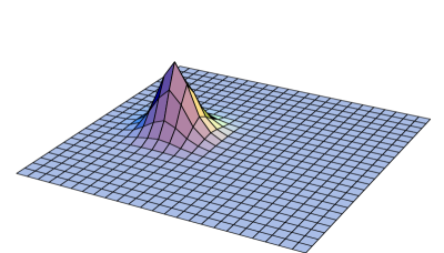
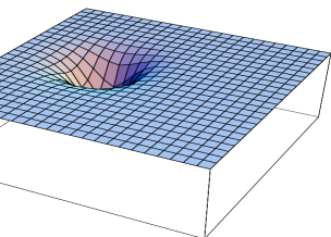
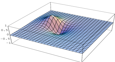
Figure 2: A charge 1 configuration on a $16^{4}$ lattice with the holonomies fixed to be trivial in one direction and maximally non-trivial in the other three directions, generated from a random start first being cooled with $\varepsilon=1$ to just above the one-instanton action, after which 80 sweeps of $\varepsilon=-1$ cooling were applied. We plot the Polyakov loop for two relevant directions, in a plane through the center of the instanton. In this plane the action density is shown in the middle.

With periodic boundary conditions we cannot keep the holonomies in the various compact directions fixed. We anticipate on the basis of the caloron studies that the constituent nature comes out best in case these holonomies are maximally non-trivial. One sure way to enforce non-trivial holonomy, as has been implemented in the finite temperature cooling studies [24], is by choosing appropriate fixed boundary conditions for the time-like links. On a symmetric box there is no preferred direction that plays the role of the imaginary time and Polyakov loops in all other directions are expected to behave similarly. Unlike at finite temperature, the holonomies in the space directions can now also be non-trivial. The most efficient way to fix the holonomy in the direction $\mu$ to $V_{\mu}$ is to take at $x_{\nu}=1$ (for $\nu\neq\mu$) all links $U_{\mu}(x)$ to be independent of the remaining three coordinates, and equal to $\bar{U}_{\mu}$ such tat $V_{\mu}=\bar{U}_{\mu}^{N_{\mu}}$. In Ref. [25] these holonomies were shown to play a role in fixing instanton moduli on the torus. For the cases studied there, the holonomies are mapped to constituent locations under the Nahm transformation. The choice of holonomy indeed strongly influences the local behaviour of the Polyakov loop. When the holonomy is non-trivial there is a characteristic “dipole” structure, but for trivial holonomy the structure is like a “monopole”, as illustrated in Fig. 2.

Due to the fixed boundary conditions one can not expect to be able to find exactly self-dual configurations, but we can again use over-improved cooling to attempt to separate constituents. The behaviour of the Polyakov loop did show that over-improved cooling has the desired effect, but we could not reach the stage where isolated action density lumps were revealed.

2.2 Adiabatic Cooling

In our search for constituents at low temperatures, we can make use of our knowledge at finite temperature, starting with a configuration that has well localized constituents. Subsequently the temperature is lowered in small steps, after each step applying ((over)-improved) cooling to re-adjust the configuration to a (near) solution. We call this process adiabatic cooling. Implementing this by adding a time slice to the lattice to lower the temperature, one has to worry how to extend the configuration to this additional slice, and whether the (discrete) change in temperature is not too big a perturbation. Both of these problems are solved when using anisotropic couplings on a symmetric lattice to implement finite temperature [13], since the anisotropy can be changed continuously. It is for this reason we introduced $\xi_{\mu}$ in Eq. (2). In this form all aspect ratios can be changed continuously. With $a_{\mu}\equiv a/\sqrt{\xi}_{\mu}$ the expansion of $S(\varepsilon)$ in Eq. (2) is as given in Eq. (3). We fix $\prod_{\mu}\xi_{\mu}=1$, such that when approximating the sum over the lattice points by an integral the leading term correctly corresponds to $-{\scriptstyle{{1\over 2}}}\int d^{4}x{\rm Tr}F_{\mu\nu}^{2}(x)$, since the proper volume element of a lattice cell is $\prod_{\mu}a_{\mu}=a^{4}$.

For finite temperature the $\xi_{\mu}$ are as usual parameterized by one anisotropy parameter $\xi$, with $\xi_{0}=\xi^{\scriptstyle{{3\over 2}}}$ and $\xi_{i}=\xi^{-{\scriptstyle{{1\over 2}}}}$. This implies that the lattice spacing in the time direction is a factor $\xi$ smaller than in the space direction, $a_{t}=a_{s}/\xi$ (or $a_{0}=a_{i}/\xi$), such that a lattice of size $N_{s}^{4}$ with an anisotropy parameter $\xi$ is equivalent to a lattice of size $N_{t}\times N_{s}^{3}$, with $N_{t}=N_{s}/\xi$. Our studies for isotropic lattices at finite temperature are with a size $4\times 16^{3}$. This would therefore be equivalent to results on a lattice of size $16^{4}$ with an anisotropy parameter $\xi=4$. Reducing $\xi$ to 1 under adiabatic cooling gives results on isotropic lattices of size $16^{4}$, which is the situation implied when we talk about zero temperature.

In our adiabatic cooling studies we used two methods to create the initial configurations at finite temperature. The simplest is to take an exact infinite volume and finite temperature continuum solution with the desired properties, naively discretized on the anisotropic lattice (by approximating the path ordered integral for the gauge field along the link by 30 steps of equal length), and performing a number of cooling sweeps to adjust it to periodic boundary conditions. The other method is first to use the results obtained from cooling on an isotropic but asymmetric lattice to get the desired finite temperature lattice configuration (e.g. using over-improvement to separate the constituents). This configuration can then be put on the finer anisotropic lattice by splitting the time-like links in $\xi=N_{s}/N_{t}$ equal factors and for the space-like links by using a geodesic interpolation on the group manifold,

$$U_{0}^{\prime}({\vec{x}},\xi(x_{0}-1)+k) = \left[U_{0}({\vec{x}},x_{0})\right]^{\frac{1}{\xi}},\quad\qquad\qquad k=1,\ldots,\xi,$$

$$U_{i}^{\prime}({\vec{x}},\xi(x_{0}-1)+k) = \left[U_{i}({\vec{x}},x_{0}+1)U^{-1}_{i}({\vec{x}},x_{0})\right]^{\frac{k-1}{\xi}}U_{i}({\vec{x}},x_{0}).$$ (4)

Again, some cooling sweeps are needed to relax the configuration to a solution on the anisotropic lattice. Both methods work equally well to find a starting configuration at finite temperature on the anisotropic lattice with well-separated constituents.

Figure 3: Starting from a continuum caloron solution with well-separated lumps, discretized on the anisotropic lattice and adjusted by 100 $\varepsilon=-10$ cooling sweeps, we performed the adiabatic cooling by reducing $\xi$ from 4 to 1, through $\xi=2\sqrt{2}$, 2 and $\sqrt{2}$, applying between each of the 4 steps 100 $\varepsilon=-10$ cooling sweeps. Shown is on the left the action density and on the right the Polyakov loop in the time direction along a line through the constituent locations. The dotted, dashed and full curves are for $\xi=4$, 2 and 1, respectively.

For charge 1, discretizing the infinite volume caloron solution is more convenient in making finite temperature configurations with well separated constituents due to the charge 1 obstruction on a torus. This was used to generate Fig. 3. We observe that each of the two separate lumps is growing in accordance of what would happen in the infinite volume when lowering the temperature. Increasing overlap leads to increasing non-static behaviour, but before the constituents become localized in all four directions, they have formed a single instanton lump.

As before, the behaviour of the Polyakov loop still allows us to identify the constituent locations. The fact that these come a little bit closer under the process of adiabatic cooling is mainly due to the obstruction for having exact solutions of charge 1 on a torus. There are two ways to avoid this finite volume obstruction, either by using higher topological charge or by the use of twisted boundary conditions, discussed in the next two sections.

3 Higher Charge Configurations

First we study in more detail the caloron moduli space at finite temperature. The interest here is two-fold. In our analytic studies we have seen that well separated constituents become point like [17] (i.e. spherically symmetric BPS monopoles [5]), but a full analytic understanding on the moduli space is not yet available. Properly manipulating $\varepsilon$ in our cooling studies, configurations can be found where the constituents are well-separated and are arbitrarily positioned. An example of a charge 3 caloron solution with non-trivial holonomy is shown in Fig. 4. One clearly distinguishes the 6 constituents, 3 of positive and 3 of negative magnetic charge.

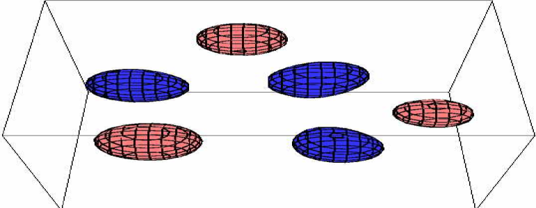
Figure 4: Example of a charge 3 caloron solution with ${\scriptstyle{{1\over 2}}}{\rm Tr}{{\cal P}_{\infty}}=-0.126$ on a $4\times 16^{3}$ lattice obtained from $\varepsilon=-1$ cooling. Shown are the surfaces where half the trace of the Polyakov loop takes on the values $0.5$ (light, red) and $-0.65$ (dark, blue), corresponding respectively to the constituent monopoles with positive and negative magnetic charge.

Next we study what happens at finite temperature under extended over-improved cooling. Oppositely charged constituents are known to be repelled and to become of equal mass under this cooling [16]. It is therefore natural to expect that constituents with equal charges are attracted. We should emphasize here again that this force is exclusively due to the lattice artifacts. It offers us an opportunity to move around in the moduli space. It should be understood though that the control one has is limited, since only one parameter $\varepsilon$ is available to manipulate all (non-trivial) moduli.

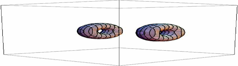
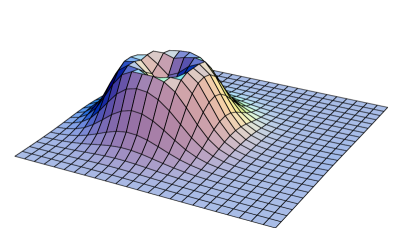
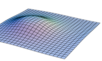
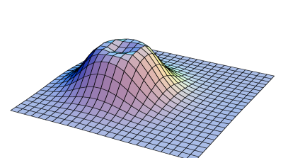
Figure 5: A charge 2 caloron with ${\rm Tr}{{\cal P}_{\infty}}=0$ on a $4\times 16^{3}$ lattice obtained from a Monte Carlo generated configuration at $4/g^{2}=2.2$. We first went down to slightly above the 2 instanton action with $\varepsilon=1$. After that many thousands of $\varepsilon=-2$ cooling sweeps (followed by 500 with $\varepsilon=0$) were performed. This gives the finite volume modification of the so-called “rectangular” solution constructed in Ref. [17]. Shown is a suitable surface of constant action density for the double doughnut structure, as well as (clockwise) the action density, the periodic zero-mode density and the Polyakov loop. The latter three are shown on a plane through the doughnut which supports the periodic zero-mode. The other doughnut seen by the action density and the anti-periodic zero-mode has the sign of the Polyakov loop inverted, but is not seen by the periodic zero-mode.

Nevertheless, this provided us with sufficient control to find for charge 2 that both constituents with the same charge will approach each other. Ultimately they will be on top of each other, forming the doughnut structure characteristic of the axially symmetric charge 2 monopole solutions [26]. Another characteristic of these solutions is the double zero in the Higgs field as reflected here in the behaviour of the Polyakov loop. At the same time the two doughnuts, which have opposite magnetic charge, are repelled and will be placed as far apart as is allowed by the finite volume. This is illustrated in Fig. 5.

Next we applied adiabatic cooling to the configuration in Fig. 5. Under very long over-improved cooling this configuration is actually reaching the exact charge 2 self-dual constant curvature solution that can exist on a symmetric torus [27, 28]. For other aspect ratios constant curvature solutions exist as well, but are in general no longer self-dual and thus unstable [28], or at best marginally stable at non-trivial holonomy [29, 30]. An expansion in the aspect ratio was performed in Ref. [31] to investigate to which type of a self-dual configuration these constant curvature solutions deform. We will not discuss this here in greater detail, but we did see similar extended structures in case $\xi$ was close to 1. The analysis in Ref. [31] was for the self-dual constant curvature solution of topological charge 1/2, based on suitably chosen twisted boundary conditions (in the 0-3 and 1-2 planes only), with the sides of the four dimensional box satisfying $L_{0}L_{3}=L_{1}L_{2}$. To get the case we studied, one combines four of these boxes to a symmetric box with no twisted boundary conditions.

Although these constant curvature configurations are rather special to the finite volume, it is nevertheless clear what gives rise to these extended structures, when one attempts to separate constituents. Lowering the temperature their size increases. For the symmetric box this size becomes of the order of (half) that of the volume, as this is the only length scale in the system when viewing a constituent in isolation. On the other hand the separation between the constituents can not get bigger than the size of the volume. The constituents are therefore bound to overlap, and in general will show a single instanton peak, which increases in height with decreasing constituent separation. Apart from exceptional cases, built from periodic arrays of charge 1/2 instantons [19] as discussed before, well-separated constituents do not reveal well-localized lumps of fractional topological charge, despite the fact that the underlying constituent description seems undeniable, as revealed by the behaviour of the Polyakov loop. An interesting question is now whether for these very extended structures the chiral fermion zero-modes still follow the underlying gluonic distribution. At finite temperature these zero-modes are exponentially localized to the cores of the constituents [17]. At zero temperature there can be no exponential localization in the classical background field. From this point of view it is interesting to study the zero-modes for the self-dual charge 2 constant curvature solution. These were constructed before in the context of the Nahm transformation [32]. For the sum of the two zero-mode densities see Fig. 6.

As we can see from this figure the zero-modes do in general not have constant density, but can of course also not be considered to be localized. As already mentioned in the case of finite temperature, the zero-modes depend on the choice of boundary conditions for the fermions. These can be periodic up to an arbitrary phase $\exp(2\pi iz_{\mu})$, here in each of the four directions, which is equivalent to adding $-2\pi iz_{\mu}\Eins_{n}/L_{\mu}$ to the gauge field, as is customary in formulating the Nahm transformation [1, 22]. In the natural basis used in Ref. [32] the two zero-modes shift in opposite directions as a function of $z_{\mu}$ and happen to have the same shape. We give the sum of the zero-mode densities in the $0$-$3$ plane for the two cases described in the caption of Fig. 6 (a slightly better “localization” can be found in the $0$-$1$ plane [33]).

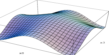
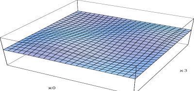
Figure 6: Sum of the two exact zero-mode densities for a charge 2 constant curvature configuration. The flux has non-zero components in the 1-2 and 0-3 planes. The result is plotted as a function of $x_{0}$ and $x_{3}$ for $x_{1}=x_{2}=z_{1}=z_{2}=0$, on the left at $z_{0}=z_{3}=0$ (the two zero-mode densities fall on top of each other) and on the right at $z_{0}=z_{3}=0.25$ (the two zero-modes densities are shifted by half a period in the $x_{0}$ and $x_{3}$ directions relative to each other).

One might argue that it is not a surprise to ultimately end up in the least localized configuration possible for the symmetric box under adiabatic cooling, since our starting point was (what we believe to be) the least localized configuration allowed at finite temperature, as shown in Fig. 5. To check that in a symmetric box the constituents indeed become as big as (half) the volume, we instead start at finite temperature with a well-localized configuration. To do this we could take an infinite volume charge 2 analytic solution with four well-separated constituents, that still fits sufficiently well into the finite volume under consideration. The most suitable configuration for this purpose is the so-called “crossed” configurations considered in Ref. [17], without a net dipole moment. But rather than following the cumbersome procedure of putting this exact charge 2 solution on the lattice, we make use of the efficiency of cooling to quickly settle down to a nearby solution. We thus take a charge 1 caloron solution whose two constituents are separated by half a period (i.e. 8 lattice spacings, twice the period in the imaginary time direction), and add to this gauge field the same solution rotated by 180 degrees and shifted perpendicular to its axis over half a period. As had been discussed extensively for the continuum in Ref. [34], this gives rise to would-be Dirac strings becoming visible, i.e. carrying action density. When simply adding two self-dual solutions, this is certainly the most conspicuous source for the violation of self-duality. Nevertheless, we have seen that cooling very quickly removes these would-be Dirac strings and automatically performs the exponential fine-tuning that would have been required in the continuum (the coarseness of the lattice in this respect has its advantages now).

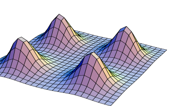
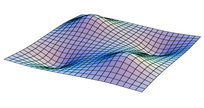
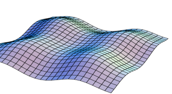
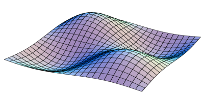
Figure 7: The result of adiabatic cooling, starting at finite temperature with two charge 1 calorons in the “crossed” configuration (see the text) on a $16^{4}$ lattice with $\xi=4$ after 1000 cooling sweeps with $\varepsilon=0$. The finite temperature solution is presented in the top two figures. The left plot shows the action density integrated over time, the right plot the Polyakov loop in the time direction, both in the $y$-$z$ plane at $x=8$ (where all constituents lie by construction). We changed $\xi$ through $2\sqrt{2}$, 2, $\sqrt{2}$ to reach 1, at each of these applying 1000 cooling sweeps with $\varepsilon=0$. The result at $\xi=1$ is given in the bottom two figures (showing the same quantities as above).

The starting configuration is shown in the top row of Fig. 7, based on improved ($\varepsilon=0$) cooling to stabilize to an exact solution (the finite volume modification of the analytic solution for the appropriate “crossed” configuration [17]). Starting from this optimally localized configuration we apply the adiabatic cooling method and find that the lumps grow and inevitably overlap, giving rise to extended structures, see the bottom row of Fig. 7. It is important to note we used $\varepsilon=0$ cooling so as to avoid the cooling to change the moduli of the self-dual solution (other than by the changing temperature). This was also to prevent being “attracted” to the constant curvature configuration, although we observed that actually the result in Fig. 7 forms a local minimum for the over-improved action. For the action density we show in this figure only the density integrated along the time direction, in the plane going through the constituents. Initially, at finite temperature the configuration is static. After the adiabatic cooling this is no longer the case. Among any of the two dimensional slices to be considered no localized structures were found. It would not serve a purpose to illustrate this here in further detail, but the structures we found look quite similar in nature to those shown in Ref. [31]. We also looked at the periodic and anti-periodic (w.r.t. “time”) zero-modes to verify the absence of localized structures.

Therefore, well-localized lumps at zero temperature for these low-charge self-dual backgrounds can only be found as instantons, even though it is clear that these are build from constituents of fractional topological charge. On the basis of the caloron solutions at finite temperature, a good guess is that the size $\rho$ of the instanton is related to the distance $d$ between its constituents as $\hat{d}=\pi\hat{\rho}^{2}$, where $\hat{d}=d/L$ and $\hat{\rho}=\rho/L$. This indeed provides a good explanation for all the features we found, also when using twisted boundary conditions to be discussed in the next section.

4 Twisted Boundary Conditions

In this section we consider (minimally) twisted boundary conditions, such that it does not affect the topological charge sectors. This is called orthogonal twist, and it is best described by the fact that doubling the box in just one of the coordinate directions removes the twist (and of course doubles the topological charge). The main reason for considering these boundary conditions is to avoid the obstruction for exact charge 1 solutions [35]. This way we can be assured that the cooling only affects the distance between the constituents [16].

First we consider the case of finite temperature with twist $\vec{k}$ in the time direction (i.e. a center flux of $k_{j}$ units in each of the $0$-$j$ planes), performing many more cooling sweeps (tens of thousands) than were considered in Ref. [16]. One would expect that the fixed point under over-improved cooling would be two constituents maximally separated, i.e. by half the size of the box. Somewhat surprisingly this turned out not to be the case and the constituents started to get closer together again “across the boundary” with further over-improved cooling. This seems in contradiction with the fact that constituents of opposite magnetic charge repel each other under over-improved cooling. Ultimately we reached the situation where the two constituents actually met and formed a doughnut structure characteristic of two coinciding magnetic monopoles of the same charge, as shown in Fig. 8 for $\vec{k}=(1,0,0)$. Indeed, like-charge constituents attract as we have seen in the previous section. We can only conclude that in the process of separating the constituents the magnetic charge of one must have changed relative to the other constituent. Recalling that the sign of the magnetic charge is correlated to the sign of the Polyakov loop observable, this behaviour is related to the fact that the Polyakov loop is anti-periodic in certain directions.

That the twisted boundary conditions interfere with the notion of magnetic and electric charge is also seen from the charge 1/2 instanton at finite temperature, which for all practical purposes behaves as a single constituent monopole as demonstrated in Ref. [25]. At first sight this seems impossible, because a net electric or magnetic charge cannot occur in a box with periodic boundary conditions. In this sense twisted boundary conditions play a similar role as C-periodic boundary conditions introduced in Ref. [36].

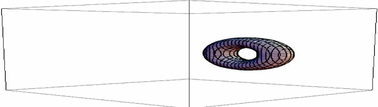
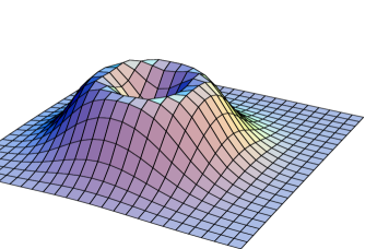
Figure 8: A charge 1 configuration on a $4\times 16^{3}$ lattice with twisted boundary conditions in the time direction, $\vec{k}=(1,0,0)$. It was obtained from a configuration, first cooled down with $\varepsilon=1$ to slightly above the one-instanton action, applying $10^{4}$ cooling sweeps with $\varepsilon=-10$ (500 cooling sweeps with $\varepsilon=0$ were finally applied to bring it close to the continuum). The constituents had been pushed so far apart that one of them effectively changed its electric and magnetic charge. The doughnut characteristic for two coinciding magnetic monopoles, with its symmetry axis along $\vec{k}$, gives the ultimate fixed-point under over-improved cooling. The right plot shows an action density contour plot of the doughnut, on the left the action density is plotted over the $y$-$z$ plane slicing the doughnut in two. Gluing two of these boxes along the $\vec{k}$ direction can be compared to Fig. 5.

We may construct a finite volume caloron by putting two boxes with topological charge 1/2 next to each other, such that the twist in the space direction cancels. This is precisely where the constituents are maximally separated and where their charge is ambiguous. When this caloron configuration is approached from a localized instanton, whose constituents are pushed apart by over-improved cooling, they would be assigned opposite magnetic charge. On the other hand, when approached from the doughnut configuration (achieved by ordinary cooling as the reverse of over-improved cooling), they would be assigned equal magnetic charge.

We also studied these twisted boundary conditions for the symmetric box. Here it is of course a matter of convention what we call the time direction. With respect to that arbitrary direction we took for the twist $\vec{k}=(1,1,1)$. We started from a localized charge one instanton. Over-improved cooling will automatically start to separate the constituents. We follow this to the point where the constituents are close to maximally separated as allowed by the box, in which case we can actually distinguish two lumps in the action density, which we plot in Fig. 9 along the line connecting the two constituents (based on an interpolation of the lattice data).

Figure 9: Results obtained with cooling on a $12^{4}$ lattice with twist in the time direction given by $\vec{k}=(1,1,1)$, starting from a random configuration. We first applied 1000 $\varepsilon=1$ cooling sweeps to go down to slightly above the one-instanton action. We plot the action density (left) and the square of half the trace of the Polyakov loop (right) along the line connecting the two constituents, every time adjusting to the continuum by 500 $\varepsilon=0$ additional cooling sweeps. Each curve, with constituents pushed further apart, is obtained after ($1000,2000,2000,44000$) additional $\varepsilon=-10$ cooling sweeps.

We find that only for the maximal separation two individual lumps are visible in the action density, but that this requires fine-tuning of the placing of these constituents; even then the lumps are as big as (half) the volume and cannot be considered localized. We have also plotted the square (due to the anti-periodicity) of half the trace of the Polyakov loop which allows us to clearly localize the separated lumps.

5 Cooling Histories

In this section we will show how cooling histories can be used to establish the existence of fractionally charged lumps. It is based on analyzing the action and topological charge as measured at plateaux, of which there can be many within a given cooling run. A plateau is defined as the point of inflection for the action as a function of the cooling sweeps (i.e. when the decrease per step becomes minimal) [7]. On the one hand, localized lumps of fractional topological charge can annihilate with another lump with the opposite fractional topological charge. This would change the overall action (always measured in units of the 1 instanton action) by twice the value of this topological charge (ranging between 0 and 2 depending on the holonomy, but typically around 1), and leave the topological charge unchanged. This can thus be easily distinguished from the annihilation of an instanton and anti-instanton, for which the action always changes by two units. On the other hand two of these lumps with the same sign for their fractional topological charge, but opposite magnetic and electric charge, can come together and form a localized instanton, which subsequently shrinks under cooling (in this section we always use $\varepsilon=1$) and then falls through the lattice. In this case both the topological charge and the action changes by one unit.

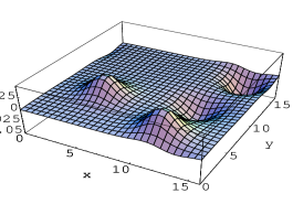
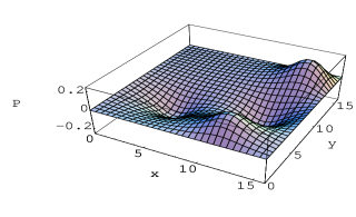
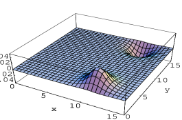
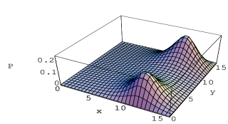
Figure 10: Example for annihilation of constituents with opposite fractional topological charge on a $4\times 16^{3}$ lattice generated from a configuration just below $T_{c}$ with ordinary cooling. Shown are, for two consecutive plateaux, the topological charge density (left) and the Polyakov loop (right) in the $x$-$y$ plane, averaged over $z$ (and $t$, though the configurations are nearly static). The annihilation is between constituents with opposite magnetic, but equal electric charge and equal Polyakov loop.

Examples for the annihilation of constituents of opposite topological charge have already been discussed in Ref. [7, 37]. Here we present two more interesting cases. Fig. 10 shows how such pairs of constituents with opposite fractional topological charge (bottom row) typically come from a caloron and an anti-caloron (top row), after annihilation of the complementary pair. In Fig. 11 we present another example in the sector with topological charge $-1$, consisting of one close pair of constituents that forms an anti-caloron, and a pair of well-separated constituents with opposite fractional topological charge. As an inset we show a surface with constant topological charge density.

Im$\,\lambda$
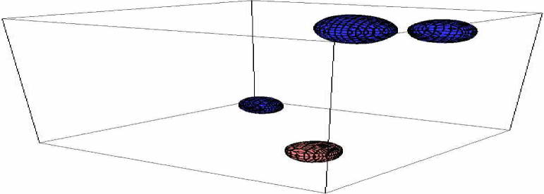
                                                                                                       $P\!=\!1\quad~{}P\!=\!-1$
                                                                                         $P=-1$
                                                                                              $P=-1$
                                                                                          Re$\,\lambda$

Figure 11: Example of a plateau configuration on a $4\times 16^{3}$ lattice (with $S=1.92$ units and ${\scriptstyle{{1\over 2}}}{\rm Tr}{{\cal P}_{\infty}}=-0.22$) before annihilation of the two bottom constituents in the inset (light (red) and dark (blue) shading distinguishes positive from negative topological charge). The Polyakov loop at the center of each of the constituents is indicated by $P=\pm 1$. The crosses give the low-lying eigenvalues $\lambda$ of the clover-improved Wilson-Dirac operator with periodic boundary conditions in time. The two curves trace the two near zero-modes from their value with anti-periodic (left) boundary conditions to the periodic (right) case (the squares correspond from left to right with $n$=$5,4,3,2,1,0$, defining the phase $\exp(2\pi in/10)$ for the fermion boundary conditions).

The colour distinguishes between the three constituents with negative and one constituent with positive topological charge. At the next plateau (reached after 236 additional cooling sweeps, not shown), the bottom pair has annihilated and the constituents of the anti-caloron came closer. Fig. 11 also shows the fermion spectrum for the first plateau. Crosses indicate the low-lying eigenvalues for the Wilson-Dirac operator for fermion boundary conditions that are periodic in time. The three lowest eigenvalues are traced as a function of the phase of the fermion boundary conditions, moving from anti-periodic (left) to periodic (right) boundary conditions. The imaginary part of the exact zero-mode stays zero as it should, whereas near zero-modes move away from zero.

The (exact positive chirality) periodic zero-mode is localized to the constituent with $P=1$ for both plateaux. With anti-periodic boundary conditions the (exact positive chirality) zero-mode for the second plateau “sees” the one remaining constituent with $P\!=\!-1$. However, for the first plateau there are altogether three such (exact and near) zero-modes. One of these is the exact positive chirality zero-mode guaranteed by the index theorem. It is concentrated only on the two constituents with negative topological charge and $P\!=\!-1$. The other two near zero-modes are localized on all three constituents with $P\!=\!-1$. But projection on the (nearly equal) negative and positive chirality components of the near zero-modes will localize to the appropriate constituent(s) with positive and negative topological charge.

$({\bf s})$

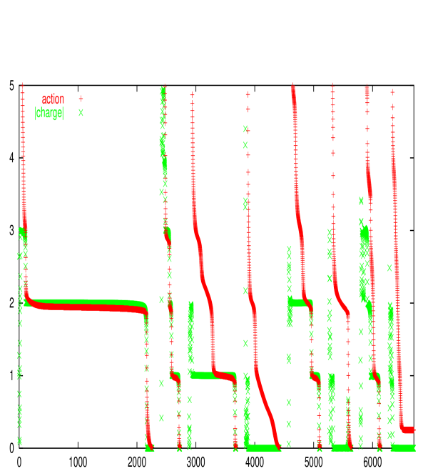
Figure 12: Sample of 8 cooling histories on a $4\times 16^{3}$ lattice at $4/g^{2}=2.2$ ($T\approx 0.8T_{c}$). Pluses give the Wilson action and crosses the absolute value of the (order $a^{2}$ improved clover averaged) topological charge. The curve “s” is an example discussed in the text.

We ran Monte Carlo on a $4\times 16^{3}$ lattice at $4/g^{2}=2.2$, extracting 50 configurations equilibrated at $T\approx 0.8T_{c}$. A sample of 8 cooling histories is shown in Fig. 12. The crosses give the (order $a^{2}$ improved clover averaged) topological charge, and the pluses the Wilson action which was used for the cooling. Much can be read off from this figure. The definition of a plateau is the point of inflection, which is also where the change in the action is slowed down, as is reflected in the greater density of symbols. The “snake-like” behaviour in the action curves (an example is indicated by “s” in the figure), along which the topological charge remains constant, represents in many cases examples where constituent annihilation takes place. This is so, because the difference in action between the consecutive plateaux (i.e. “bends”) is closer to one, rather than to two instanton units. This can be contrasted with the behaviour at low temperature ($T\approx 0.25T_{c}$) with a sample of cooling histories presented in Fig. 13, obtained on a $16^{4}$ lattice at $4/g^{2}=2.3$.

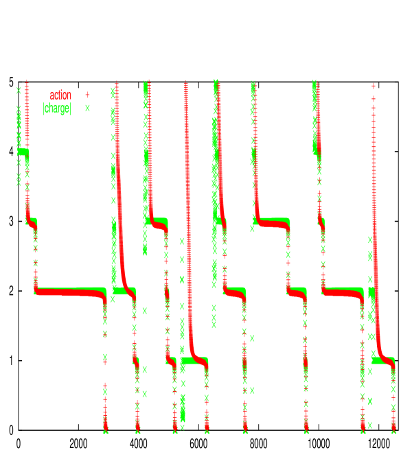
Figure 13: Sample of 8 cooling histories on a $16^{4}$ lattice at $4/g^{2}=2.3$ ($T\approx 0.25T_{c}$). The symbols are as discussed in the caption of Fig. 12.

A similar study on a $4\times 16^{3}$ lattice at $4/g^{2}=2.4$ for the deconfined phase was performed as well. In the relatively rare cases that a plateau is seen, there is no sign of constituent annihilation. This agrees with our expectations, since at trivial holonomy only one of the constituent monopoles is massive, capturing all of the action. We do find at finite temperature some plateaux below the one-instanton action, which are by now well understood as (approximate) constant magnetic field configurations [37, 30]. In the confined phase these can be stable depending on the precise value of the holonomy, and the last cooling run shown in Fig. 12 provides a clear example. The minimal value for a $4\times 16^{3}$ lattice is one quarter of the instanton action, but we found also values twice and three times that big.

We summarize our findings for the plateau analysis in a scatter plot for the decrease in action ($\Delta S$) between two plateaux, versus the absolute value of the change in the topological charge ($|\Delta Q|$), see Fig. 14.

Figure 14: Scatter plots of $|\Delta Q|$ (horizontally) versus $\Delta S$ (vertically) for (i) a $4\times 16^{3}$ lattice at $4/g^{2}=2.4$ ($T\approx 1.2T_{c}$), (ii) a $4\times 16^{3}$ lattice at $4/g^{2}=2.2$ ($T\approx 0.8T_{c}$), note the significant clustering around $\Delta S=1$, $|\Delta Q|=0$ characteristic of constituent annihilations, and (iii) a $16^{4}$ lattice at $4/g^{2}=2.3$ ($T\approx 0.25T_{c}$). Each case is based on 50 configurations.

Most points in the scatter plot are associated to the typical process of instanton disappearance, distributed around $\Delta S=|\Delta Q|=1$. The clustering of the points around $\Delta S=1$ and $|\Delta Q|=0$, absent for zero and high temperatures, is nevertheless clear evidence for the annihilation of localized constituents with opposite fractional topological charge. The action of these constituents depends on the holonomy; its fluctuations are reflected in the spread of $\Delta S$ around 1.

6 Summary and Discussion

We have analysed the constituent nature of instantons, both at finite and zero temperature. As a convenient way to describe the instanton moduli space, constituents were long ago conjectured to play a role and called instanton quarks [18]. Some early realizations in terms of instantons with topological charge $1/n$, that can exist with twisted boundary conditions [15, 19], were considered in Ref. [20] (singular solutions like merons [38] excluded). Constituents with arbitrary fractional topological charge were realized at finite temperature in the background of non-trivial holonomy [3]. When well-separated these are described in a precise way by BPS monopole configurations [5]. In the confined phase, where on average the holonomy is maximally non-trivial, the topological charge fraction is on average $1/n$.

Here we have investigated in what sense self-dual solutions of higher topological charge are made up of constituents and how the latter overlap. Furthermore, we have followed what happens to the constituents in self-dual solutions when adiabatically lowering the temperature. As deduced from the behaviour of the Polyakov loop, constituents remain present despite the fact that they cannot reveal themselves as isolated action density lumps. At zero temperature these constituents become massless and are obviously not dilute, even though instantons can still be seen as the “hadrons” made out of these constituents. The name instanton quarks is therefore quite appropriate, and the possibility of confinement described in terms of a high density ensemble of these constituents becomes an appealing one [39]. This would in some sense be the “dual” of deconfinement for high density quark matter, even though it remains difficult to quantify this point of view.

Our study has its limitations, since we mainly probe self-dual configurations through the cooling studies we performed. In earlier phases of the cooling, annihilations of constituents (and instantons) of opposite topological charge do of course take place. We have even used this to deduce the presence of constituents from just studying the cooling histories. This, however, only works when the constituents are relatively dilute and well-localized. When not dilute, any extended and overlapping structures of opposite topological charge will be removed under cooling before being able to be identified. More suitable for dynamical studies is the use of chiral fermion zero-modes to identify topological structures, as was studied extensively in Refs. [8, 10, 40]. To identify the constituents one makes use of the fact that when well-separated the localization of the zero-modes depends strongly on the boundary conditions used for the fermions [9]. At finite temperature these findings agree beautifully with the results obtained by cooling. We have demonstrated another effect that can be explained by well-separated constituents, namely that the number of near zero-modes (in a smooth, but non-selfdual background) can depend on the fermion boundary conditions.

The signature of well-localized zero-modes changing location when cycling through the fermion boundary conditions was also found at zero-temperature [10]. A good measure for the localization [8] is the inverse participation ratio, $I\equiv V\sum_{x}\rho^{2}(x)$, where $\rho(x)$ is the zero-mode density. The bigger $I$ is, the more localized is the zero-mode. This can be contrasted with a constant zero-mode density for which $I=1$. On average, at finite temperature [8] $I$ is indeed considerably larger than at zero temperature [10], but in the latter case values of $I$ as big as 20 or more are still seen to occur for cases where zero-modes jump over distances as large as half the size of the volume when cycling through the boundary conditions. On the other hand, at low temperatures the inverse participation ratios never reached values above 2 for the zero-modes with maximally separated constituents, as part of self-dual configurations.

These studies, using zero-modes as a filter for Monte Carlo generated configurations, have not yet provided other independent means to distinguish whether a zero-mode is associated to a constituent of fractional topological charge or to an instanton with integer topological charge. The possibility that the zero-modes are localized to instantons (formed from closely bound constituents) and jump between well-separated instantons, rather than well-separated isolated constituents, was discussed in Ref. [41]. It was found that at finite temperature this is unlikely to occur, but it could not be ruled out for zero temperature. The analysis assumes the constituents to be relatively dilute and well-localized, neither of which seems to be the case at zero temperature. The argument relies on the fact that typically there will be many topological lumps of either sign, when no cooling is applied to the Monte Carlo generated configurations. For configurations with exactly one negative chirality zero-mode, one minimally requires the presence of $n$ instantons and $n-1$ anti-instantons in order for the negative chirality zero-mode to be able to visit $n$ different locations, as would be the case for an SU($n$) caloron with well-separated constituents.

In a random medium of topological lumps the mechanism of localization of the zero-modes could very well be similar to Anderson localization [42]. In such a case one perhaps should expect a dependence on the fermion boundary conditions, even when constituents remain well hidden inside instantons. In the case that instantons form a dense ensemble, this is similar to the statement that it is impossible to determine which set of instanton quarks form an instanton. Still, the essential fact remains that the boundary conditions determine to which type of instanton quark the zero-mode localizes. That some of the zero-modes, if associated to fractionally charged lumps, are more localized than we observed in the studies presented here can have a dynamical origin. Further work will be required to understand all this in more detail, but it seems legitimate to conclude that constituents are here to stay, and may well play an important role in our understanding of confinement.

References

- [1] W. Nahm, Self-dual monopoles and calorons, in: Lect. Notes in Physics. 201, eds. G. Denardo, e.a. (1984) p. 189.
- [2] K. Lee and P. Yi, Phys. Rev. D56 (1997) 3711 [hep-th/9702107]; K. Lee, Phys. Lett. B426 (1998) 323 [hep-th/9802012]; K. Lee and C. Lu, Phys. Rev. D58 (1998) 025011 [hep-th/9802108].
- [3] T.C. Kraan and P. van Baal, Phys. Lett. B428 (1998) 268 [hep-th/9802049]; Nucl. Phys. B533 (1998) 627 [hep-th/9805168]; Phys. Lett. B435 (1998) 389 [hep-th/9806034].
-
[4]
G. ’t Hooft, Nucl. Phys. B79 (1974) 276;
A.M. Polyakov, JETP Lett. 20 (1974) 194. -
[5]
E.B. Bogomol’ny, Sov. J. Nucl. Phys. 24 (1976) 449;
M.K. Prasad and C.M. Sommerfield, Phys. Rev. Lett. 35 (1975) 760. - [6] G. ’t Hooft, Nucl. Phys. B190 (1981) 455; Physica Scripta 25 (1982) 133.
- [7] E.-M. Ilgenfritz, B.V. Martemyanov, M. Müller-Preussker, S. Shcheredin and A.I. Veselov, Phys. Rev. D66 (2002) 074503 [hep-lat/0206004].
- [8] C. Gattringer and S. Schaefer, Nucl. Phys. B654 (2003) 30 [hep-lat/0212029].
- [9] M. García Pérez, A. González-Arroyo, C. Pena and P. van Baal, Phys. Rev. D60 (1999) 031901 [hep-th/9905016]; M.N. Chernodub, T.C. Kraan and P. van Baal, Nucl. Phys. B(Proc.Suppl.) 83 (2000) 556 [hep-lat/9907001].
- [10] C. Gattringer and R. Pullirsch, Phys. Rev. D69 (2004) 094510 [hep-lat/0402008].
- [11] E.M. Ilgenfritz, B.V. Martemyanov, M. Müller-Preussker and A.I. Veselov, Phys. Rev. D69 (2004) 114505 [hep-lat/0402010].
- [12] M. García Pérez, A. González-Arroyo, J. Snippe and P. van Baal, Nucl. Phys. B413 (1994) 535 [hep-lat/9309009].
- [13] F. Karsch, Nucl. Phys. B205 (1982) 285.
- [14] M. Fujisaki et al. [QCD-TARO Collaboration], Nucl. Phys. B[Proc. Suppl.] 53 (1997) 426 [hep-lat/9609021]; M. García Pérez and P. van Baal, Phys. Lett. B392 (1997) 163 [hep-lat/9610036].
- [15] G. ’t Hooft, Nucl. Phys. B153 (1979) 141; Acta Physica Aust. Suppl. XXII (1980) 531.
- [16] M. García Pérez, A. González-Arroyo, A. Montero and P. van Baal, JHEP 06 (1999) 001 [hep-lat/9903022].
- [17] F. Bruckmann, D. Nógrádi and P. van Baal, Nucl. Phys. B666 (2003) 197 [hep-th/0305063]; hep-th/0404210 (to appear in Nucl. Phys. B).
- [18] A.A. Belavin, V.A. Fateev, A.S. Schwarz and Y.S. Tyupkin, Phys. Lett. B83 (1979) 317.
- [19] M. García Pérez, A. González-Arroyo and B. Söderberg, Phys. Lett. B235 (1990) 117.
- [20] A. González-Arroyo, P. Martínez and A. Montero, Phys. Lett. B359 (1995) 159 [hep-lat/9507006]; A. González-Arroyo and P. Martínez, Nucl. Phys. B459 (1996) 337 [hep-lat/9507001]; A. González-Arroyo and A. Montero, Phys. Lett. B387 (1996) 823 [hep-th/9604017].
- [21] B. Berg, Phys. Lett. B104 (1981) 475; E.-M. Ilgenfritz, M.L. Laursen, G. Schierholz, M. Müller-Preussker and H. Schiller, Nucl. Phys. B268 (1986) 693; J. Hoek, M. Teper and J. Waterhouse, Nucl. Phys. B288 (1987) 589.
- [22] P.J. Braam and P. van Baal, Comm. Math. Phys. 122 (1989) 267.
- [23] C. Taubes, J. Diff. Geom. 19 (1984) 517.
- [24] E.-M. Ilgenfritz, M. Müller-Preussker, and A.I. Veselov, in: Lattice fermions and structure of the vacuum, eds. V. Mitrjushkin and G. Schierholz (Kluwer, 2000), 345 [hep-lat/0003025]. E.-M. Ilgenfritz, B.V. Martemyanov, M. Müller-Preussker and A.I. Veselov, Nucl. Phys. B(Proc.Suppl.)94 (2001) 407 [hep-lat/0011051].
- [25] M. García Pérez, A. González-Arroyo, C. Pena and P. van Baal, Nucl. Phys. B564 (2000) 159 [hep-th/9905138].
- [26] P. Forgács, Z. Horváth and L. Palla, Nucl. Phys. B192 (1981) 141; M.F. Atiyah, and N.J. Hitchin, The Geometry and Dynamics of Magnetic Monopoles, (Princeton Univ. Press, 1988).
- [27] G. ’t Hooft, Comm. Math. Phys. 81 (1981) 267.
- [28] P. van Baal, Comm. Math. Phys. 94 (1984) 397.
- [29] M. García Pérez and P. van Baal, Nucl. Phys. B429 (1994) 451 [hep-lat/9403026]; P. van Baal, Nucl. Phys. B(Proc.Suppl.)47 (1996) 326 [hep-lat/9508019].
- [30] E.-M. Ilgenfritz, M. Müller-Preussker, B.V. Martemyanov and P. van Baal, Phys. Rev. D69 (2004) 097901 [hep-lat/0402020].
- [31] M. García Pérez, A. González-Arroyo and C. Pena, JHEP 0009 (2000) 033 [hep-th/0007113].
- [32] P. van Baal, Nucl. Phys. B(Proc.Suppl)49 (1996) 238 [hep-th/9512223].
- [33] M. García Pérez, Zero modes on constant curvature backgrounds, talk presented at the workshop “The QCD Vacuum from a Lattice Perspective”, 29-31 July 2004, Regensburg, Germany.
- [34] F. Bruckmann and P. van Baal, Nucl. Phys. B645 (2002) 105 [hep-th/0209010].
- [35] P. Braam, A. Maciocia and A. Todorov, Inv. Math. 108 (1992) 419.
- [36] A.S. Kronfeld and U.J. Wiese, Nucl. Phys. B357 (1991) 521.
- [37] E.-M. Ilgenfritz, M. Müller-Preussker, B.V. Martemyanov and A. Veselov, Eur. Phys. J. C34 (2004) 439 [hep-lat/0310030].
- [38] V. de Alfaro, S. Fubini and G. Furlan, Phys. Lett. B65 (1976) 163; C.G. Callan, R. Dashen and D.J. Gross, Phys. Lett. B66 (1977) 375.
- [39] F. Bruckmann, D. Nógrádi and P. van Baal, Acta Phys. Polon. B34 (2003) 5717 [hep-th/0309008].
- [40] C. Gattringer, Phys. Rev. D67 (2003) 034507 [hep-lat/0210001].
- [41] F. Bruckmann, M. García Pérez, Nógrádi and P. van Baal, Nucl. Phys. B(Proc. Suppl.)129 (2004) 727 [hep-lat/0308017].
- [42] P.W. Anderson, Phys. Rev. 109 (1958) 1492.