Monopole gas in three dimensional SU(2) gluodynamics

Abstract

We study properties of the Abelian monopoles in the Maximal Abelian projection of the three dimensional pure SU(2) gauge model. We match the lattice monopole dynamics with the continuum Coulomb gas model using a method of blocking from continuum. We obtain the Debye screening length and the monopole density in continuum using numerical results for the lattice density of the (squared) monopole charges and for the monopole action. The monopoles treated within our blocking method provide about $75\%$ contribution to the non–Abelian Debye screening length. We also find that monopoles form a Coulomb plasma which is not dilute.

I Introduction

According to the dual superconductor mechanism DualSuperconductor the confinement of quarks in non–Abelian gauge theories is caused by the monopole–like configurations of the gluonic fields. These configurations can be identified with the help of the Abelian projection method AbelianProjections . The basic idea behind this method is to fix partially the non–Abelian gauge symmetry up to an Abelian subgroup. If the original non–Abelian gauge group is compact (like the SU(N) group) then the residual Abelian symmetry group is compact as well. The compactness of the Abelian group guarantees the existence of the monopoles.

In the low temperature phase of the four dimensional SU(N) gauge model the monopoles are condensed MonopoleCondensation in agreement with the dual superconductor mechanism DualSuperconductor . The condensation leads to the appearance of the dual Meissner effect and, as a result, to the formation of the chromoelectric string between fundamental sources of the chromoelectric field (quarks). Consequently, the quarks get confined. Moreover, the Abelian monopoles are in the so-called Maximal Abelian projection MaA make to make a dominant contribution to the zero temperature string tensionAbelianDominance (for a review, see Ref. Review ).

At the critical temperature, $T=T_{c}$, the monopole condensate disappears and at higher temperatures the quarks are no more confined. The vacuum in the deconfinement phase is filled by the static monopoles which can not lead to the confinement of the static quarks. However, the absence of the color confinement at high temperatures does not mean that the high temperature physics is perturbative. Indeed, even at $T>T_{c}$ the quarks running in the spatial directions are still confined due to existence of the ”spatial string tension” (this is a coefficient in front of the area term of large spatial Wilson loops). The spatial string tension is a non–perturbative quantity which is dominated by contributions of the static monopoles according to Ref. AbelianDominanceT .

The physics of the static monopoles in the high temperature SU(2) gauge model was investigated in Ref. JHEP using the method called blocking from continuum (BFC). This method resembles the idea of the blocking of the continuum fields to the lattice BlockingOfFields . In general the BFC procedure allows us to match lattice results to the continuum model without going to a deep continuum limit. For example, the BFC method clearly shows JHEP that in the continuum limit the static monopoles in the high temperature SU(2) gluodynamics are described by the three dimensional Coulomb gas model. Another example is the zero–temperature 4D SU(2) gluodynamics in which the value of the monopole condensate can be obtained with the help of the BFC method CondensateBFC . Being encouraged by these results, we apply the BFC method to the monopoles in the three-dimensional SU(2) gluodynamics. The confinement mechanism in this model based on the Abelian monopole dynamics was previously discussed both within analytical ref:three:dim:analyt and numerical Bornyakov ; ref:three:dim:numerical frameworks.

The plan of the paper is as follows. In Section II we briefly recall the results of the Ref. JHEP for the lattice density of the (squared) monopole charge and for the monopole action expressed via parameters of the continuum Coulomb gas model. In Section III we study the lattice action and the lattice density of the monopoles in the pure $3D$ SU(2) gauge model. Using the BFC method we get density of the monopoles and the monopole contribution to the magnetic screening length in the continuum limit. Our conclusion is presented in the last Section.

II Lattice monopoles from continuum monopoles

The standard way to identify the lattice monopoles in Monte Carlo simulations is to use the DeGrand-Toussaint construction DGT which calculates the magnetic flux coming out of lattice 3D cells (cubes). The magnetic charges obtained in this way are conserved and quantized. The properties of the lattice monopoles should obviously depend on the physical size, $b$, of the lattice cell (below we call these lattice objects as ”lattice monopoles of the size $b$”). To get the properties of the monopoles in continuum one should send the size of the lattice cells to zero, $b\to 0$, what is usually a difficult numerical problem. The BFC method allows to get the properties of the monopoles in continuum (”continuum monopoles”) using the results obtained on the lattice with a finite lattice spacing.

The idea behind the BFC method is to treat each lattice 3D cell as a ”detector” of the magnetic charges of the continuum monopoles. If the continuum monopole is located inside a lattice 3D cell then the DeGrand-Toussaint method detects an existence of a lattice monopole inside this cell. If the size, $b$, of the lattice cell is finite then two or more continuum monopoles may be located inside the cell. The fluctuations of the monopole charges of the lattice cells must depend on the properties of the continuum monopoles. As a result, the lattice observables – such as the vacuum expectation value of the lattice monopole density (or, the lattice action) – must carry information about dynamics of the continuum monopoles. The observables should depend not only on the size of the lattice cell, $b$, but also on features of the continuum model which describes the monopole dynamics.

To avoid misunderstanding we would like to stress from the very beginning the difference between various lattice monopole sizes $b$. As we mentioned above, we call the size of the lattice 3D cell – used for detection of the monopoles – as ”the size of the lattice monopole”. This should be distinguished from the physical radius, $r_{0}$, of the monopole core FiniteRadius which is obviously independent on the size of the lattice ”detector”. In this paper we disregard the existence of the monopole core and consider the continuum monopoles as point–like objects. Thus, we get the finite–sized lattice monopoles by blocking the point–like continuum monopoles to the lattice.

Below we describe briefly the techniques which appear in the BFC method. Let us consider a three–dimensional lattice with a finite lattice spacing $b$ which is embedded in the continuum space-time. The cells of the lattice are defined as follows:

$$C_{s}=\Biggl{\{}b\Bigl{(}s_{i}-\frac{1}{2}\Bigr{)}\leq x_{i}\leq b\Bigl{(}s_{i}+\frac{1}{2}\Bigr{)}\,,\quad i=1,2,3\Biggr{\}}\,,$$ (1)

where $s_{i}$ is the lattice dimensionless coordinate and $x_{i}$ corresponds to the continuum coordinate.

The magnetic charge, $k_{s}$, inside the lattice cell $C_{s}$ is

$$k_{s}=\int\limits_{C_{s}}\mbox{d}^{3}x\,\rho(x)\,,\qquad\rho(x)=\sum_{a}q_{a}\,\delta^{(a)}(x-x^{(a)})\,,$$ (2)

where $\rho(x)$ is the density of the continuum monopoles, $x_{a}$ and $q_{a}$ is the position and the charge (in units of a fundamental magnetic charge, $g_{M}$) of $a^{\mathrm{th}}$ continuum monopole. In three dimensions the monopoles are instanton–like objects and the monopole trajectories have zero dimensionality (points). Basic properties of the lattice monopoles are the same as the ones of the continuum monopoles: the charge $k_{s}$ is quantized, $k_{s}\in{Z\!\!\!Z}$, and conserved in the three-dimensional sense:

$$\sum_{s\in\Lambda}k_{s}\equiv\int\limits_{V}\mbox{d}^{3}x\,\rho(x)=0\,.$$

Here $\Lambda$ and $V$ denote the lattice and the continuum volume occupied by the lattice, respectively.

In the BFC method various properties of the lattice monopoles such as the lattice monopole density, correlators of the lattice monopole charges, the effective lattice monopole action etc. can be calculated in a continuum monopole model using Eq. (2) as a definition of the lattice monopole charge. In this paper we suppose that the dynamics of the continuum monopoles is governed by the $3D$ Coulomb gas model:

$${\cal Z}=\sum\limits_{N=0}^{\infty}\frac{\zeta^{N}}{N!}\Biggl{[}\prod\limits^{N}_{a=1}\int\mbox{d}^{3}x^{(a)}\sum\limits_{q_{a}=\pm 1}\Biggr{]}\exp\Bigl{\{}-\frac{g^{2}_{M}}{2}\sum\limits_{\stackrel{{\scriptstyle a,b=1}}{{a\neq b}}}^{N}q_{a}q_{b}\,D(x^{(a)}-x^{(b)})\Bigr{\}}\,.$$ (3)

The Coulomb interaction in Eq.(3) is represented by the inverse Laplacian $D$, $-\partial^{2}_{i}D(x)=\delta^{(3)}(x)$, and $\zeta$ is the fugacity parameter.

The model (3) does not exist without properly defined ultraviolet cut–off. Indeed, the self–energy of the point–like monopoles is a linearly divergent function. As a result, the fugacity must be renormalized, $\zeta_{\mathrm{ren}}=\zeta\cdot\exp\{g^{2}_{m}/(8\pi\,r_{0})\}$, where $r_{0}$ is the ultraviolet cut–off. In our case this cut–off is given by the size of the monopole core which is of the order of 0.05 fm at zero temperature FiniteRadius . For simplicity we omit the subscript ”ren” in the renormalized fugacity below.

The magnetic charges in the Coulomb gas (3) are screened: at large distances the two–point charge correlation function is exponentially suppressed, $\langle\rho(x)\rho(y)\rangle\sim\exp\{-|x-y|/\lambda_{D}\}$. Here $\lambda_{D}$ is the Debye screening length Polyakov ,

$$\lambda_{D}=\frac{1}{g_{M}\sqrt{\rho}}\,,$$ (4)

which is inversely proportional to the Debye screening mass, $M_{D}=\lambda^{-1}_{D}$. The density of the continuum monopoles in the leading order is related to fugacity as Polyakov $\rho=2\zeta$.

In Ref. JHEP the lattice monopole action, $S_{mon}(k)$, and the v.e.v. of the squared magnetic charge, $\langle k^{2}_{s}\rangle$, were calculated starting from the Coulomb gas model (3). In the low-density approximation the leading order contribution to the (squared) density of the monopole charges is JHEP :

$$\langle k^{2}(b)\rangle=\frac{1}{L^{3}}\,\langle\sum_{s\in\Lambda}k^{2}(s)\rangle\equiv\int_{C_{s}}\mbox{d}^{3}x\int_{C_{s}}\mbox{d}^{3}y\,\langle\rho(x)\,\rho(y)\rangle=\rho\,b^{3}\,P(M_{D}\,b)\,,$$ (5)

where in the thermodynamic limit (an infinite–volume lattice) the function $P$ is

$$P(\mu)=1-\mu^{2}\,\int\frac{\mbox{d}^{3}\,q}{{(2\pi)}^{3}}\,\frac{1}{q^{2}+\mu^{2}}\,\prod^{3}_{i=1}{\Biggl{[}\frac{2\sin(q_{i}/2)}{q_{i}}\Biggr{]}}^{2}\,.$$ (6)

The finite–volume analogue of Eq. (6) can be obtained by the standard substitution:

$$q_{i}\to\frac{2\pi k_{i}}{L_{i}}\,,\qquad\int\limits^{\infty}_{-\infty}\frac{\mbox{d}q_{i}}{2\pi}\to\frac{1}{L_{i}}\sum\limits_{k_{i}\in{Z\!\!\!Z}}\,,$$ (7)

where $L_{i}$ is the lattice size (in units of the lattice spacing) in $i^{\mathrm{th}}$ direction.

The reason why the density of the squared magnetic charges, $\langle k^{2}_{s}\rangle$, is used instead of the standard definition of the density, $\langle|k_{s}|\rangle$, is simple: an analytical treatment of $\langle|k_{s}|\rangle$ is obviously much more difficult compared to that of the quantity $\langle k^{2}_{s}\rangle$.

The explicit behavior of the lattice monopole density (5) as the function of $b$ can be obtained in the limit of large lattice monopoles JHEP ,

$$\langle k^{2}\rangle=C_{1}\,\rho\,\lambda_{D}\,b^{2}\cdot\left[1+O\left({\left(\lambda_{D}/b\right)}^{2}\right)\right]\,,\qquad b\gg\lambda_{D}\,,$$ (8)

as well as in the case of small monopoles,

$$\langle k^{2}\rangle=\rho\,b^{3}\cdot\left[1+C_{2}\,\rho\,{(b/\lambda_{D})}^{2}\,+O\left({\left(b/\lambda_{D}\right)}^{4}\right)\right]\,,\qquad b\ll\lambda_{D}\,,$$ (9)

where $C_{1}\approx 2.94$ and $C_{2}\approx 0.148$.

The proportionality of the density $\langle k^{2}\rangle$ to $b^{2}$ in large–$b$ region has a simple explanation JHEP . In a random gas of continuum monopoles we would obviously get $\langle k^{2}\rangle\sim\rho\,b^{3}$. Due to the Debye screening in the Coulomb monopole gas the monopoles separated from the boundary of the cell by the distance larger than $\lambda_{D}$, do not contribute to $\langle k^{2}\rangle$. Consequently, the $b^{3}$ proportionality for the random gas turns into $\lambda_{D}b^{2}$ in the Coulomb gas and we get $\langle k^{2}\rangle\propto\rho\,\lambda_{D}\,b^{2}$.

In the small $b$ region the density of the squared lattice monopole charges is equal to the density of the continuum monopoles times the volume of the cell. This is natural, since the smaller volume of the lattice cell, $b^{3}$, the smaller chance for two continuum monopoles to be located at the same cell. Therefore each cell predominantly contains not more that one continuum monopole, which leads to the relation $k^{2}_{s}=|k_{s}|=0,1$. As a result we get $\langle k^{2}\rangle\to\rho_{latt}(b)\to\rho\,b^{3}$ in the limit $b\to 0$.

Analogously one can get that in the large-$b$ region the action of the monopole is given by the lattice Coulomb action JHEP ,

$$S_{mon}(k)=\frac{1}{\rho\,\lambda_{D}}\cdot\frac{1}{b^{2}}\cdot\sum\limits_{s,s^{\prime}}k_{s}\,D_{s,s^{\prime}}\,k_{s^{\prime}}+\cdots\,,\qquad b\gg\lambda_{D}\,,$$ (10)

where the coefficient in front of the lattice monopole action is inversely proportional to $b^{2}$.

III Numerical results

We have simulated the pure SU(2) gauge model with the standard Wilson action $S=-1/2\sum_{P}{\mathrm{Tr}}\,U_{P}$, where $U_{P}$ is the plaquette matrix constructed from the gauge link fields, $U_{l}$. We have generated 200 configurations of the gauge fields for each chosen value of the coupling constant, $\beta=2.083,2.5,3,3.47,3.75,4.5,5,6,6.56,9,12,14.5$, on the lattice $48^{3}$. To study the Abelian monopole dynamics we perform Abelian projection in the Maximally Abelian (MA) gauge MaA for each $SU(2)$ configuration. The MA gauge fixing condition is the maximization of the quantity $R$,

$$\max\limits_{\Omega}R[U^{(\Omega)}]\,,\qquad R[U]={\mathrm{Tr}}\sum_{s,\mu}[U_{\mu}(s)\sigma_{3}U_{\mu}^{\dagger}(s+\hat{\mu})\sigma_{3}].$$ (11)

under the $SU(2)$ gauge transformations, $U\to U^{(\Omega)}=\Omega^{\dagger}U\Omega$. The gauge fixing condition (11) is invariant under an Abelian subgroup of the group of the $SU(2)$ gauge transformations. Thus the condition (11) corresponds to the partial gauge fixing, $SU(2)\to U(1)$.

After the MA gauge fixing, the Abelian, $\{u_{\mu}(s)\}$, and non–Abelian $\{\tilde{U}_{\mu}(s)\}$ link fields are separated:

$$\tilde{U}_{\mu}(s)=C_{\mu}(s)u_{\mu}(s)\,,\quad C_{\mu}(s)=\left(\begin{array}[]{cc}\sqrt{1-|c_{\mu}(s)|^{2}}&-c_{\mu}^{\ast}(s)\\ c_{\mu}(s)&\sqrt{1-|c_{\mu}(s)|^{2}}\end{array}\right)\,,\quad u_{\mu}(s)=\left(\begin{array}[]{cc}e^{i\theta_{\mu}(s)}&0\\ 0&e^{-i\theta_{\mu}(s)}\end{array}\right).$$ (16)

The vector fields $C_{\mu}(s)$ and $u_{\mu}(s)$ transform like a charged matter and, respectively, a gauge field under the residual U(1) symmetry. Next we define a lattice monopole current (DeGrand-Toussaint monopole) DGT . Abelian plaquette variables $\theta_{\mu\nu}(s)$ are written as

$$\theta_{\mu\nu}(s)=\theta_{\mu}(s)+\theta_{\nu}(s+\hat{\mu})-\theta_{\mu}(s+\hat{\nu})-\theta_{\nu}(s)\,,\qquad(-4\pi<\theta_{\mu\nu}(s)\leq 4\pi).$$ (17)

It is decomposed into two terms using integer variables $n_{\mu\nu}(s)$:

$$\theta_{\mu\nu}(s)\equiv\bar{\theta}_{\mu\nu}(s)+2\pi n_{\mu\nu}(s)\,,\qquad(-\pi<\bar{\theta}_{\mu\nu}(s)\leq\pi).$$ (18)

Here $\bar{\theta}_{\mu\nu}(s)$ is interpreted as an electromagnetic flux through the plaquette and $n_{\mu\nu}(s)$ corresponds to the number of Dirac string piercing the plaquette. The lattice monopole current is defined as

$$k(s)=\frac{1}{2}\epsilon_{\nu\rho\sigma}\partial_{\nu}n_{\rho\sigma}(s+\hat{\mu})\,.$$ (19)

In order to get the lattice density for the monopoles of various sizes, $b$, we perform numerically the blockspin transformations for the lattice monopole charges. The original model is defined on the fine lattice with the lattice spacing $a$ and after the blockspin transformation, the renormalized lattice spacing becomes $b=na$, where $n$ is the number of steps of the blockspin transformations. The continuum limit is taken as the limit $a\to 0$ and $n\to\infty$ for a fixed physical scale $b$.

The monopoles on the renormalized lattices (”extended monopoles”, Ref. ExtendedMonopoles ) have the physical size $b^{3}$. The charge of the $n$–blocked monopole is equal to the sum of the charges of the elementary lattice monopoles inside the $n^{3}$ lattice cell:

$$k^{(n)}(s)=\sum_{i,j,l=0}^{n-1}k\bigl{(}ns+i\hat{\mu}+j\hat{\nu}+l\hat{\rho}\bigr{)}\,.$$

For the sake of simplicity we omit below the superscript $(n)$ while referring to the blocked currents. We perform the lattice blocking with the factors $n=1\dots 12$. All dimensional quantities below are measured in units of the string tension, $\sigma$, the values of which are taken from Ref. Teper:StringTensions ; Teper:Glueball .

We show the density of the squared monopole charges (normalized by the factor $b^{2}$) in Figure 1 as a function of the scale $b$ for various blocking factors, $n$.

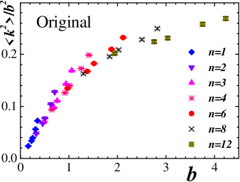
Figure 1: The density of the squared lattice monopole charges, $\langle k^{2}_{s}\rangle$, divided by $b^{2}$ as a function of $b$ for various blocking steps $n$ ($b$ is given in units of the string tension, $\sigma$).

One can easily see from this Figure that the density shows only an approximate scaling: the data depends not only on $b=an$, but also on the fine lattice spacing, $a$, and the blocking factor, $n$, separately. The violation of the $b$–scaling – being much bigger then the error bars of the data – strongly affects the physical results.

The origin of the $b$–scaling violation is in the presence of the ultraviolet lattice artifacts which express themselves in the form of the tightly bound monopole–anti-monopole pairs (magnetic dipoles). These dipoles are living on the fine lattice and typical distance between the constituents of the these dipoles is of the order of the fine lattice spacing, $a$. Thus, in the continuum limit these dipoles must disappear. However, on the finite lattices they affect the results drastically.

In order to get rid of the ultraviolet artifacts we have removed the tightly–bound dipole pairs from all configurations using a simple numerical algorithm. Namely, we remove a magnetic dipole if it is made of a monopole and an anti-monopole which are touching each other (i.e., this means that the centers of the corresponding cubes are located at the distance smaller or equal than $\sqrt{3}a$). Note, that we first apply this procedure to the elementary $a^{3}$–monopoles, and only then we perform the blockspin transformations. Below we discuss the results obtained for the monopole ensembles with the artificial UV–dipoles removed.

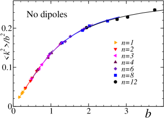
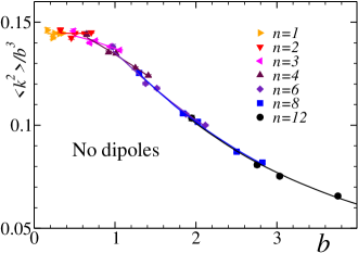
(a)	(b)

Figure 2: The density of the squared monopole charges, $\langle k^{2}_{s}\rangle$, with the UV dipoles removed. The density is normalized (a) by $b^{2}$ and (b) by $b^{3}$. The fits by the function (5) are shown by dashed lines for each value of the blocking step, $n$.

In Figure 2(a) we show the density of the squared monopole charges as a function of the scale $b$ for various values of the blocking factor, $n$. The density is normalized by the factor $b^{2}$. One can see that the $b$-scaling violations are very small. As the blocking size $b$ increases the slope of the ratio $\langle k^{2}_{s}\rangle/b^{2}$ becomes less steep. This behavior is in a qualitative agreement with the prediction from the Coulomb gas model (8) which says that in the high–$b$ limit the ratio $\langle k^{2}_{s}\rangle/b^{2}$ should converge to a constant.

On the other hand the quantity $\langle k^{2}_{s}\rangle$ should be proportional to $b^{3}$ in the small–$b$ region (9). One can indeed observe from Figure 2(b) that the ratio $\langle k^{2}_{s}\rangle/b^{3}$ does tend to a constant at small $b$. Note that there is a small scaling violation in this region which is due to the presence of the lattice artifacts at the scale $b\sim a$. In order to get artifact–free results we will use below large–$b$ monopoles.

The values of the parameters of the Coulomb gas model in the continuum limit, Eq. (3), can be obtained by fitting the numerical results for $\langle k^{2}_{s}\rangle$ by the theoretical prediction (5),(7). Technically, for each value of the blocking step, $n$, we have a set of the data corresponding to different values of the lattice coupling $\beta$, and, consequently, to different values of $b=n\cdot a(\beta)$. Note that by fixing $n$ we simultaneously fix the extension of the coarse lattice, $L/n$, in units of $b$. The size of the coarse lattice enters in Eq. (7). We fit the set of the data for the fixed blocking step $n$. The best fit curves are shown in Figures 2(a) and (b) by dashed lines. The quality of the fit is very good, $\chi^{2}/d.o.f.\sim 1$.

The density fits give the values of the continuum monopole density, $\rho^{(n)}$, and the Debye mass, $M^{(n)}_{D}$, which are shown in Figures 3(a,b) as a function of blocking step $n$. All these results are given in units of the string tension.

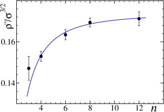
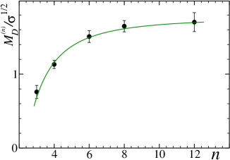
(a)	(b)

Figure 3: (a) The density of the continuum monopoles, $\rho$, and (b) the Debye screening mass, $M_{D}$, obtained with the help of the fits of the $n$–blocked squared monopole density by function (5). The large–$n$ extrapolation (20) is shown by solid lines.

The influence of the finite lattice spacing should vanish in the limit of large $b$, or, in our case, in the limit of large $n$: $\lim_{n\to\infty}{\cal O}^{(n)}={\cal O}^{\mathrm{ph}}$, where ${\cal O}$ stands for either $\rho$ or $M^{D}$ and the superscript ”ph” indicate the artifact–free physical value. We found that for $n>2$ the dependence of both $\rho$ and $M_{D}$ on the blocking size $n$ can be approximately described as

$${\cal O}^{(n)}={\cal O}^{\mathrm{ph}}+{\mathrm{const}}\cdot n^{-2}\,,$$ (20)

The extrapolation (20) is shown in Figure 3. We get the physical values for the monopole density $\rho$ and the Debye screening mass $M_{D}$ coming from the Coulomb gas model (here and below we omit the superscript ”ph” for the extrapolated values):

$$\rho\,/\sigma^{3/2}=0.174(2)\,,\qquad M_{D}\,/\sigma^{1/2}=1.77(4)\,.$$ (21)

The value of $M_{D}$ may be treated as the ”monopole contribution to the Debye screening mass”.

The self–consistency check of our approach can be done with the help of the quantity

$$C=\frac{M_{D}\,\sigma}{\rho}\,,$$ (22)

which is known to be equal to eight ($C^{\mathrm{CG}}=8$) in the low density limit of the Coulomb gas model Polyakov . In Figure 4 we plot our numerical result for $C$ as a function of $n$.

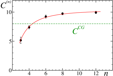
Figure 4: The same as in Figure 3 but for the ratio (22). The dashed line corresponds to the low density limit of Coulomb Gas model Polyakov , $C^{\mathrm{CG}}=8$.

The large–$n$ extrapolation (20) gives

$$C=10.1(1)\,,\qquad{\it i.e.}\qquad\frac{C}{C^{\mathrm{CG}}}=1.26(3)\,.$$ (23)

The quantity $C$ is about $25\%$ larger than the one predicted by the Coulomb gas model in the low monopole density approximation, $C^{\mathrm{CG}}_{sp}=8$. The discrepancy is most likely explained by the invalidity of the assumption that the monopole density is low. Indeed, the low–density approach requires for the monopole density to be much lower than a natural scale for the density, $g^{6}$ (remember that the coupling $g$ has the dimensionality $mass^{1/2}$). The requirement $\rho\ll g^{6}$ can equivalently be reformulated as $\rho/M_{D}^{3}\gg 1$, which means that the number of the monopoles in a unit Debye volume, $\lambda_{D}^{3}\equiv M_{D}^{-3}$, must be high. Taking the numerical values for $\rho$ and $M_{D}$ from Eq. (21) we get: $\rho/M_{D}^{3}\approx 0.03\ll 1$. Thus, the low–density assumption is not valid in the 3D SU(2) gluodynamics. However, the discrepancy of $25\%$ observed in the quantity $C$, Eq. (23), is a good signal that the Coulomb gas model may still provide us with the predictions valid up to the specified accuracy.

One can compare our result for the monopole density, Eq. (21), with the result obtained by Bornyakov and Grigorev in Ref. Bornyakov , $\rho^{\mathrm{BG}}=2^{-7}(1\pm 0.02)\,g^{6}$. Using the result of Ref. Teper:StringTensions , $\sqrt{\sigma}=0.3353(18)\,g^{2}$, we get the value $\rho^{\mathrm{BG}}/\sigma^{3/2}=0.207(5)$, which is close to our independent estimation in the continuum limit (21): $\rho/\rho^{\mathrm{BG}}=0.83(4)$. The result of Ref. Bornyakov is about $20\%$ higher than our estimation for the monopole density. Thus, although the condition of the low monopole density approximation is strongly violated, the BFC method (based on the dilute gas approximation) gives the value of the monopole density which is consistent with other measurements.

It is interesting to compare the result for the screening mass (21) with the lightest glueball mass measured in Refs. Teper:StringTensions ; Teper:Glueball , $M_{O^{++}}=4.72(4)\,\sqrt{\sigma}$. In the Abelian picture, the mass of the ground state glueball obtained with the help of the correlator,

$$\langle F^{2}_{\mu\nu}(0)\,F^{2}_{\alpha\beta}(R)\rangle={\mathrm{const.}}\,e^{-M_{O^{++}}\,R}+\dots\,,$$

must be twice bigger than the Debye screening mass, $2M_{D}/M_{O^{++}}=1$, where the Debye mass is given by the following correlator

$$\langle F_{\mu\nu}(0)\,F_{\mu\nu}(R)\rangle={\mathrm{const.}}\,e^{-M_{D}\,R}+\dots\,.$$

The comparison of our result (21) with the result of Refs. Teper:StringTensions ; Teper:Glueball gives $2M_{D}/M_{O^{++}}=0.75(4)$. The deviation is of the order of $25\%$ similarly to case of the quantity $C$.

Let us also compare our result for the monopole contribution to the Debye screening mass, Eq. (21), with the direct measurement of the Debye mass in 3D SU(2) gauge model made in Ref. Karsch , $m^{SU(2)}_{D}/\sqrt{\sigma}=1.39(9)$. The values agree with each other within the $25$ per cent: $m_{D}/m^{SU(2)}_{D}=1.27(11)$. Approximately the same accuracy is observed in the four–dimensional SU(2) gauge theory for the monopole contribution to the fundamental string tension ref:Bali .

Finally, we have made the cross–check of our result by a numerical calculation of the effective monopole action. We used an inverse Monte-Carlo algorithm described in Ref. Yazawa and we used the following form of the trial action:

$$S_{mon}(k)=f_{1}\cdot\sum\limits_{s}k^{2}_{s}+f_{Coul}\cdot\sum\limits_{s,s^{\prime}}k_{s}\,D_{s,s^{\prime}}\,k_{s^{\prime}}\,.$$ (24)

The choice of this type of the trial action is motivated by the following reasons. From the point of view of reliability of the results the data is most valuable in the large-$b$ region since the subtraction of the ultraviolet monopoles can not change the infrared physics. In this region the action is expected to be given by the Coulomb term (10). On the other hand the subtraction of the ultraviolet monopoles must affect the ultraviolet (or, local) terms in the monopole action. Thus we added to the trial action (24) the most local term with the coupling $f_{1}$. The role of this term is to take into account the effects which are caused by the monopole subtraction.

We depict the coupling $f_{1}$ and the product $b^{2}\,f_{Coul}$ as a function of $b$ in Figures 5(a,b), respectively.

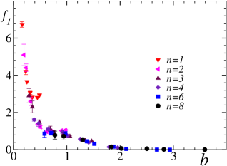
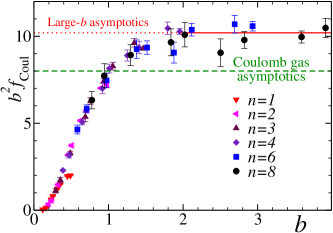
(a)	(b)

Figure 5: The coupling $f_{1}$ and the product $b^{2}\,f_{Coul}$ of the action (24) $vs.$ $b$ for each value of the blocking step, $n$.

The strong coupling region with $\beta\leqslant 3.0$ was not included into these figures due to large finite size effects. Indeed, in this case $a\sqrt{\sigma}\gtrsim 0.6$ which implies that $aM_{D}\approx 1$ (here we used the value of $M_{D}\equiv\lambda_{D}^{-1}$ obtained from the fits of the monopole density (21)).

Note that small–$n$ results are more sensitive to the subtraction of the ultraviolet magnetic dipoles. This is the reason for noticeable $b$–scaling violations around $b\sim 0.5\sigma^{-1/2}$ for $n=1$ in both Figures 5(a,b).

According to the analytical prediction (10) the product of the coupling $f_{Coul}$ and $b^{2}$ should tend to a constant in the limit $b\gg\lambda_{D}$ while the $f_{1}$–term should disappear from the action. Numerically, the coupling $f_{1}$ is diminishing as $b$ increases, as seen in Figure 5(a). One can also check numerically that this coupling is vanishing quicker than $1/b^{2}$ at $b\gtrsim 1.5\sigma^{-1/2}$. So in the large–$b$ region we are indeed left only with the lattice Coulomb term in the action. If the scale $b$ is expressed in units of the string tension then the product $b^{2}f_{Coul}(b)$ tend to the quantity (22). Figure 5(b) shows that large-$b$ plateau in distribution of $b^{2}f_{Coul}(b)$ starts from $b\gtrsim 2\sigma^{-1/2}$. Averaging the available data with $b\geqslant 2\sigma^{-1/2}$ we get $C=10.2(3)$ which is in an excellent agreement with the result (23) obtained from the monopole action.

IV Conclusions

We have shown that the dynamics of the Abelian monopoles in the three–dimensional SU(2) gauge model can be described by the Coulomb gas model. Using a novel method, called the blocking of the monopoles from continuum, we calculated the monopole density and the Debye screening mass in continuum, Eq. (21), using the numerical results for the (squared) monopole charge density. The self-consistency of the results was checked by the independent analysis of the lattice monopole action. We conclude that the Abelian monopole gas in the 3D SU(2) gluodynamics is not dilute. Nevertheless, the continuum values of the monopole density ($\rho=0.174(2)\,\sigma^{3/2}$) and the Debye screening mass ($M_{D}=1.77(4)\,\sigma^{1/2}$) – obtained with the help of the dilute monopole gas model – are consistent within the accuracy of $25\%$ with the known data obtained from independent measurements.