Perturbative determination of mass dependent renormalization and improvement coefficients for the heavy-light vector and axial-vector currents with relativistic heavy and domain-wall light quarks

Abstract

We determine the mass dependent renormalization as well as improvement coefficients for the heavy-light vector and axial-vector currents consisting of the relativistic heavy and the domain-wall light quarks through the standard matching procedure. The calculation is carried out perturbatively at the one loop level to remove the systematic error of $O(\alpha_{s}(am_{Q})^{n}a\mbox{\boldmath$p$})$ as well as $O(\alpha_{s}(am_{Q})^{n})$ ($n\geq$0), where $p$ is a typical momentum scale in the heavy-light system. We point out that renormalization and improvement coefficients of the heavy-light vector current agree with those of the axial-vector current, thanks to the exact chiral symmetry for the light quark. The results obtained with three different gauge actions, plaquette, Iwasaki and DBW2, are presented as a function of heavy quark mass and domain-wall height.

I Introduction

The study of heavy-light hadrons including a single heavy quark ($b$ or $c$) has played a central role in the particle physics. In particular, much attentions have been paid to estimating weak decay matrix elements of these hadrons to determine the Cabbibo-Kobayashi-Maskawa matrix elements. Lattice QCD simulation offers a promising method to calculate the decay amplitudes from the first principles, and a number of efforts using lattice QCD have been already made and contributed to the heavy-light physics Yamada:2002wh ; Kronfeld:2003sd .

However, the lattice calculation of the heavy-light system is not yet precise enough. Since the currently accessible inverse lattice spacing is at most $1/a\sim$3, 4 GeV, so that $am_{b,c}\ll$1 never holds, the lattice calculations suffer from sizable $O((am_{b,c})^{n})$ ($n>$1) errors. Another difficulty, though this is a rather general problem in Lattice QCD simulations of hadrons, arises from chiral extrapolations of physical quantities to their physical values ($\sim m_{u,d}$) as numerically investigated in Refs. Aoki:2003xb ; Aoki:2001yr ; Yamada:2001xp . Because of limited computational resources, we are forced to simulate light quarks much heavier than the physical light quark masses, and, then, long extrapolations are required. In addition, non-analytic behaviors of physical quantities around the massless point which chiral perturbation theory predicts make reliable extrapolations even more difficult.

One possible way to overcome the above obstacles is to combine the relativistic heavy quark Aoki:2001ra and the domain-wall light quark Kaplan:1992bt ; Shamir:1993zy ; Furman:ky to simulate heavy-light quark systems. The relativistic heavy quark Aoki:2001ra is obtained by pushing the on-shell improvement program Luscher:1984xn to the Wilson type massive fermions, and its action is equal to the Fermilab action El-Khadra:1996mp with a special choice of parameters. The relativistic heavy quark action has four parameters to be tuned, and the perturbative determination of these parameters as well as the wave function renormalization has been completed to the one-loop level so far Aoki:2003dg . As for the problem of chiral extrapolations in terms of light quark masses, we employ the domain-wall formalism for light quarks, which has already been used successfully in large scale simulations. It has been demonstrated that this formalism allows to simulate lighter quarks than the standard Wilson type quark action.

In this paper, we determine the renormalization coefficients for the heavy-light vector and axial-vector currents consisting of the relativistic heavy and the domain-wall light quarks through the standard one-loop matching. The improvement coefficients associated with the dimension four operators are evaluated to the one-loop as well. Since the obtained coefficients depend on both heavy quark mass $m_{Q}$ and domain-wall height $M_{5}$, we work out the interpolation formula to express the results as simple as possible. In this work we take three different gauge actions, the plaquette, the Iwasaki Iwasaki:1983ck and DBW2 Takaishi:1996xj ; deForcrand:1999bi , as examples. The Feynman rules and useful formula for the gauge actions are described in Ref. Aoki:2003dg in rather general manner, so we will omit that part of explanations from this paper. With the coefficients obtained here and the lattice calculations of all relevant operators, we can remove the systematic error of $O(\alpha_{s}(am_{Q})^{n}a\mbox{\boldmath$p$})$ as well as $O(\alpha_{s}(am_{Q})^{n})$ ($n\geq$0) from physical amplitudes. As for the calculational method, we completely follows that in Ref. Aoki:2004th , where the similar calculations are performed using the clover action for the light quark.

This paper is organized as follows. In Sec. II, we briefly explain the quark actions used in the following sections. In Sec.III, the definitions of the renormalization and improvement coefficients which we determine in this paper are given. Then, we give a short notice on the benefit of chiral symmetry in Sec.IV. The calculational method and the numerical results are given in Secs. V. In Sec. VI, we consider two ways to improve the convergence of the perturbative series. Concluding remarks are stated in Sec. VII. In the process of this calculation, we found that the on-shell improvement of the massive domain-wall fermions is necessary. The improvement procedure in this case is briefly explained in appendix A.

II the quark actions

II.1 The relativistic heavy quark

In this work, the heavy quark is described by the relativistic heavy quark action Aoki:2001ra ,

$$S_{Q}=\sum_{x} \!\!\!\left[\ m_{0}{\bar{Q}}(x)Q(x)+{\bar{Q}}(x)\gamma_{0}D_{0}Q(x)+\nu_{Q}\sum_{i}{\bar{Q}}(x)\gamma_{i}D_{i}Q(x)\right.$$ (1)

$$\left.-\frac{r_{t}a}{2}{\bar{Q}}(x)D_{0}^{2}Q(x)-\frac{r_{s}a}{2}\sum_{i}{\bar{Q}}(x)D_{i}^{2}Q(x)\right.$$

$$\left.-\frac{iga}{2}c_{E}\sum_{i}{\bar{Q}}(x)\sigma_{0i}F_{0i}Q(x)-\frac{iga}{4}c_{B}\sum_{i,j}{\bar{Q}}(x)\sigma_{ij}F_{ij}Q(x)\ \right].$$

The parameters appearing in the action are determined by requiring $n$-point amputated on-shell Green’s function on the lattice to be equal to the continuum one up to $O(a^{2})$. In order to obtain the improvement coefficients which are valid at an arbitrary quark mass, no expansion in $(am_{0})$ nor $1/(am_{0})$ is allowed through the calculation. By matching the two-point function (propagator) to the continuum one at tree level, the pole mass, wave function, $\nu_{Q}$ and $r_{s}$ are found to be

$$m_{Q}^{(0)} = \ln\left|\frac{m_{0}+r_{t}+\sqrt{m_{0}^{2}+2r_{t}m_{0}+1}}{1+r_{t}}\right|,$$ (2)

$$Z_{Q,{\rm latt}}^{(0)} = {\rm cosh}(m_{Q}^{(0)})+r_{t}\,{\rm sinh}(m_{Q}^{(0)}),$$ (3)

$$\nu_{Q}^{(0)} = \frac{{\rm sinh}(m_{Q}^{(0)})}{m_{Q}^{(0)}},$$ (4)

$$r_{s}^{(0)} = \frac{{\rm cosh}(m_{Q}^{(0)})+r_{t}\,{\rm sinh}(m_{Q}^{(0)})}{m_{Q}^{(0)}}-\frac{{\rm sinh}(m_{Q}^{(0)})}{\left(m_{Q}^{(0)}\right)^{2}}=\frac{1}{m_{Q}^{(0)}}(Z_{Q}^{(0)}-\nu_{Q}^{(0)}).$$ (5)

Matching the amputated three-point function (quark-gluon form factor) leads to

$$c_{E}^{(0)} = r_{t}\,\nu_{Q}^{(0)},$$ (6)

$$c_{B}^{(0)} = r_{s}^{(0)}.$$ (7)

Since $r_{t}$ is not constrained from the improvement condition, in the following we set $r_{t}$=1 for simplicity. Once the parameters have been tuned to their proper values given in eqs. (2)–(7), we can remove the systematic errors of $O((am_{Q})^{n})$ and $O((am_{Q})^{n}a\mbox{\boldmath$p$})$ ($n\geq$0) from the action.

Extending the above procedure to the one-loop level, $O(\alpha_{s}(am_{Q})^{n})$ and $O(\alpha_{s}(am_{Q})^{n}a\mbox{\boldmath$p$})$ ($n\geq$0) errors are removed. This calculation was carried out in Ref. Aoki:2003dg , and the numerical results depending on the quark mass are given in terms of an interpolation formula. Here we only quote the result of the wave function renormalization for the later use. Defining the wave function renormalization by

$$Q_{{\overline{\rm MS}}} = \sqrt{Z_{Q}(m_{Q}^{(0)})}\,Q_{\rm latt},$$ (8)

$$Z_{Q}(m_{Q}^{(0)}) = \frac{Z_{Q,{\rm latt}}(m_{Q}^{(0)})}{Z_{Q,{\rm cont}}(m_{Q}^{(0)})}=Z_{Q,{\rm latt}}^{(0)}(m_{Q}^{(0)})\,\left[1+g^{2}\bigg{(}-\frac{C_{F}}{16\pi^{2}}\ln(a^{2}\mu^{2})+\Delta_{Q}(m_{Q}^{(0)})\bigg{)}\right],$$ (9)

$\Delta_{Q}(m_{Q}^{(0)})$ is, to good precision, given by

$$\Delta_{Q}(m_{Q}^{(0)})=\Delta_{Q}(0)+\frac{\sum_{i=1}^{4}a_{i}\{m_{Q}^{(0)}\}^{i}}{1+\sum_{i=1}^{4}b_{i}\{m_{Q}^{(0)}\}^{i}},$$ (10)

where the values of $\Delta_{Q}(0)$, $a_{i}$ and $b_{i}$ ($i=1,\dots,4$) are listed in Table II of Ref. Aoki:2003dg .

It should be noted that in the massless limit all $\nu_{Q}^{(0)}$, $r_{s}^{(0)}$, $c_{E}^{(0)}$ and $c_{B}^{(0)}$ are reduced to unity (for $r_{t}$=1), and the action is reduced to the $O(a)$ improved SW quark action Sheikholeslami:1985ij . More importantly, the space-time rotational symmetry is restored in this limit to all orders of $a$ and $\alpha_{s}$.

II.2 The domain-wall quark action

As for light quarks, we take the domain-wall fermion Kaplan:1992bt ; Shamir:1993zy ; Furman:ky . More precisely, we employ the following version of the domain-wall action in this work,

$$S_{\rm DW} = \sum_{x,y}\sum_{s,t}\bar{\psi}_{s}(x)D_{\rm DW}(x,s;y,t)\psi_{t}(y),$$ (11)

$$D_{\rm DW}(x,s;y,t) = D_{\rm W}(x,y)\,\delta_{s,t}+\delta_{x,y}D_{5}(s,t),$$ (12)

$$D_{\rm W}(x,y) = \sum_{\mu}\gamma_{\mu}D_{\mu}-\frac{a}{2}\sum_{\mu}D_{\mu}^{2}-M_{5}\,\delta_{x,y},$$ (13)

$$D_{5}(s,t) = \delta_{s,t}-P_{L}\,\delta_{s+1,t}-P_{R}\,\delta_{s-1,t}+m_{f}\left[P_{L}\,\delta_{s,N_{5}}\delta_{1,t}+P_{R}\,\delta_{s,1}\delta_{N_{5},t}\right],$$ (14)

where $P_{R/L}=(1\pm\gamma_{5})/2$, and $s$ and $t$ label the coordinate of the fifth dimension running 1 to $N_{5}$. We set $N_{5}\rightarrow\infty$ throughout this paper. The physical quark field $q(x)$ is, then, constructed by

$$q(x) = P_{L}\psi_{1}(x)+P_{R}\psi_{N_{5}}(x),$$ (15)

$$\bar{q}(x) = \bar{\psi}_{1}(x)P_{R}+\bar{\psi}_{N_{5}}(x)P_{L}.$$ (16)

As long as massless quarks are concerned, this original action is enough to proceed. However, as explained in Ref. Aoki:2004th and later as well, in a part of calculations we should keep the light quark mass small but finite. Once quark masses become finite, the infrared divergences which do not exist in the continuum show up in a certain class of loop integrations due to the mismatch of dispersion relation and make perturbative matching to $O(\alpha_{s}a\mbox{\boldmath$p$})$ meaningless. To eliminate the mismatch, the original domain-wall action is required to be improved, and the improvement can be realized by simply applying the on-shell improvement program Luscher:1984xn ; Aoki:2001ra to the massive domain-wall fermion. As a consequence, it is found that we need, at least, two modifications in the original domain-wall action. First we replace the first term of eq. (13) with

$$\gamma_{0}D_{0}+\nu_{q}\sum_{i}\gamma_{i}D_{i},$$ (17)

and, then, add a new term,

$$-\frac{R_{s}}{2}\ \bar{q}(x)\ \sum_{i}D_{i}^{2}\ q(x)=-\frac{R_{s}}{2}\ \bar{\psi}_{s}(x)\ \sum_{i}D_{i}^{2}\ \left(P_{L}\ \delta_{s,N_{5}}\delta_{t,1}+P_{R}\ \delta_{s,1}\delta_{t,N_{5}}\right)\ \psi_{t}(x),$$ (18)

to the action eq. (11). Here we introduced two parameters $\nu_{q}$ and $R_{s}$, which can be tuned by following the on-shell improvement program Aoki:2001ra . As a result (see appendix A for the derivations), we obtain

$$\nu_{q}^{(0)}(m_{q}^{(0)}) = \frac{\mbox{$\sinh(m_{q}^{(0)})$}}{m_{q}^{(0)}},$$ (19)

$$R_{s}^{(0)}(m_{q}^{(0)},M_{5}) = \frac{m_{f}}{m_{q}^{(0)}\,\mbox{$\sinh(m_{q}^{(0)})$}\,(1-m_{f}^{2})}$$ (20)

$$\times\Bigg{[}\ (1+m_{f}^{2})\left(\mbox{$\cosh(m_{q}^{(0)})$}-\frac{\mbox{$\sinh(m_{q}^{(0)})$}}{m_{q}^{(0)}}\right)-2\,m_{f}\,(2-M_{5})\big{(}\,\mbox{$\sinh(m_{q}^{(0)})$}-m_{q}^{(0)}\big{)}$$

$$\hskip 17.22217pt-2\,m_{f}\,m_{q}^{(0)}\left(\mbox{$\cosh(m_{q}^{(0)})$}-\frac{(\mbox{$\sinh(m_{q}^{(0)})$})^{2}}{(m_{q}^{(0)})^{2}}\right)\ \Bigg{]},$$

where $m_{q}^{(0)}$ is the tree-level pole mass depending on $m_{f}$ and $M_{5}$, and its expression is given in eq. (94). As $m_{f}\rightarrow 0$, these parameters approach to

$$\nu_{q}^{(0)} \rightarrow 1+O(m_{f}^{2}),$$ (21)

$$R_{s}^{(0)} \rightarrow \frac{m_{f}}{3}+O(m_{f}^{3}),$$ (22)

respectively, and, thus, the action is reduced to the original one. Analytical studies of the loop integrations reveal that the tree level matching of $\nu_{q}$ and $R_{s}$ suffices to get rid of the extra infrared divergences associated with massive light quarks, so that it is not necessary to introduce terms like the clover terms in this work though to remove the $O((am_{q}^{(0)})^{n}a\mbox{\boldmath$p$})$ errors from the action throughly we still need the clover terms whose tree-level coefficients are calculated in appendix A.

For the wave function renormalization, the one for the massless domain-wall fermions is sufficient for the following calculation. The relation of the massless domain-wall quark field to the continuum one with ${\overline{\rm MS}}$ in NDR is given by

$$q_{{\overline{\rm MS}}} = \sqrt{\frac{Z_{q}(w_{0})}{(1-w_{0}^{2})\,Z_{w}(w_{0})}}\,q_{{\rm latt}},$$ (23)

$$w_{0} = 1-M_{5},$$ (24)

$$Z_{q}(w_{0}) = 1+g^{2}\left(-\frac{C_{F}}{16\pi^{2}}\ln(a^{2}\mu^{2})+\Delta_{q}(w_{0})\right),$$ (25)

$$Z_{w}(w_{0}) = 1+g^{2}\Delta_{w}(w_{0}),$$ (26)

and the numerical values of $\Delta_{q}(w_{0})$ and $\Delta_{w}(w_{0})$ for various values of $w_{0}$ ($M_{5}$) are constructed from $z_{2}({\rm DRED})$ and $\Sigma_{w}$, which are tabulated in Tables I, III and V of Ref. Aoki:2002iq for the plaquette, Iwasaki and DBW2 gauge actions respectively, through the relations,

$$\Delta_{q}(w_{0}) = \frac{C_{F}}{16\pi^{2}}z_{2}({\rm NDR})=\frac{C_{F}}{16\pi^{2}}\,\left(z_{2}({\rm DRED})+1\right),$$ (27)

$$\Delta_{w}(w_{0}) = \frac{C_{F}}{16\pi^{2}}\,\frac{2w_{0}}{1-w_{0}^{2}}\Sigma_{w}.$$ (28)

The space-time rotational symmetry is recovered in the massless limit to all orders of $a$ and $\alpha_{s}$.

III definition of the improvement coefficients

Taking into account existing symmetries such as parity, charge conjugation, etc., it is turned out that the renormalized continuum vector and axial-vector currents can be expressed in terms of $O(a)$ improved lattice operators as

$$V^{{\overline{\rm MS}}}_{\mu}(x)=Z_{V_{\mu}}^{{\overline{\rm MS}}-{\rm latt}} \!\!\!\!\left[\,{\bar{q}(x)}\gamma_{\mu}Q(x)-g^{2}c_{V_{\mu}}^{+}\partial_{\mu}^{-}\{{\bar{q}(x)}Q(x)\}-g^{2}c_{V_{\mu}}^{-}\partial_{\mu}^{+}\{{\bar{q}(x)}Q(x)\}\right.$$ (29)

$$\left.-g^{2}c_{V_{\mu}}^{L}\{{\vec{\partial}_{i}}{\bar{q}(x)}\}\gamma_{i}\gamma_{\mu}Q(x)-g^{2}c_{V_{\mu}}^{H}{\bar{q}(x)}\gamma_{\mu}\gamma_{i}\{{\vec{\partial}_{i}}Q(x)\}+O(g^{4})\right],$$

$$A^{{\overline{\rm MS}}}_{\mu}(x)=Z_{A_{\mu}}^{{\overline{\rm MS}}-{\rm latt}} \!\!\!\!\left[\,{\bar{q}(x)}\gamma_{\mu}\gamma_{5}Q(x)-g^{2}c_{A_{\mu}}^{+}\partial_{\mu}^{+}\{{\bar{q}(x)}\gamma_{5}Q(x)\}-g^{2}c_{A_{\mu}}^{-}\partial_{\mu}^{-}\{{\bar{q}(x)}\gamma_{5}Q(x)\}\right.$$ (30)

$$\left.+g^{2}c_{A_{\mu}}^{L}\{{\vec{\partial}_{i}}{\bar{q}(x)}\}\gamma_{i}\gamma_{\mu}\gamma_{5}Q(x)-g^{2}c_{A_{\mu}}^{H}{\bar{q}(x)}\gamma_{\mu}\gamma_{5}\gamma_{i}\{{\vec{\partial}_{i}}Q(x)\}+O(g^{4})\right].$$

where $\partial^{\pm}$=$\partial_{\mu}\raisebox{7.74998pt}{$\rightarrow$}\pm\partial_{\mu}\raisebox{7.74998pt}{$\leftarrow$}$, $q(x)$ and $Q(x)$ represent light and heavy quark fields defined on the lattice, respectively, and the coefficients $Z_{V_{\mu},A_{\mu}}^{{\overline{\rm MS}}-{\rm latt}}$ and $c_{V_{\mu},A_{\mu}}^{\pm,H,L}$ are the ones we determine in the following sections. While the right hand side can be written in a gauge invariant way by replacing partial derivatives with covariant derivatives, the above expression suffices for the following discussion. Although the general form given in eqs. (29) and (30) does not depend on details of the lattice actions, the coefficients $Z_{V_{\mu},A_{\mu}}^{{\overline{\rm MS}}-{\rm latt}}$ and $c_{V_{\mu},A_{\mu}}^{\pm,H,L}$ do. Since the space-time rotational symmetry is, in general, violating on the lattice unless quarks are massless, the fourth and fifth terms on the right hand side are required to improve the violation. Therefore, although the equation of motion always allows us to set $c^{H}_{V_{0},A_{0}}=c^{L}_{V_{0},A_{0}}=0$ and we take this, it never means that the space-time rotational symmetry is recovered in the temporal component of the currents.

IV benefit of chiral symmetry

Here let us mention an advantage of using lattice chiral fermions to describe the light quark in heavy-light system by taking the heavy-light vector and axial-vector currents as examples. The similar discussion is made in Ref. Becirevic:2003hd , where the renormalization of the static-light current is calculated using the overlap fermion for the light quark. The authors of Ref. Gulez:2003uf also mentioned the similar point in the calculation with the NRQCD heavy and the naive light quarks.

Now let us consider a system including $N_{f}$=2 massless light quarks $q^{i}(x)$ ($i=1,2$), described by the lattice fermions with the exact chiral symmetry, and one heavy quark $Q(x)$. An infinitesimal flavor non-singlet axial transformation is defined by

$$\delta_{A}\,q^{i}(x) = iw^{a}(x)\,\frac{(\tau^{a})^{ij}}{2}\,\gamma_{5}\,q^{j}(x),$$ (31)

$$\delta_{A}\,\bar{q}^{i}(x) = \bar{q}^{j}(x)iw^{a}(x)\,\frac{(\tau^{a})^{ji}}{2}\,\gamma_{5},$$ (32)

where $i$ and $j$ are the flavor indexes and run 1 to $N_{f}$, and $\tau^{a}$ is the Pauli matrix. Hereafter we take an arbitrary transformation parameter $w^{a}(x)$ as

$$w^{a}(x)=\left\{\begin{array}[c]{ll}\delta_{a,3}&\mbox{for $x$ $\in$ R}\\ 0&\mbox{otherwise}\end{array}\right.,$$ (35)

where $R$ is a certain space-time region with smooth boundary $\partial R$. The exact chiral symmetry for the light quarks ensures the existence of the conserved axial-vector current. Using this fact, we can derive the following axial Ward-Takahashi identity on the lattice

$$\langle 0|\ i\int_{\partial R}\!\!d\sigma_{\mu}(y)\,A^{3,\rm ll}_{\mu}(y)\,{\cal O}_{\rm int}\,{\cal O}_{\rm ext}\ |0\rangle=\langle 0|\ (\delta_{A}{\cal O}_{\rm int})\,{\cal O}_{\rm ext}\ |0\rangle,$$ (36)

where $A^{3,\rm ll}_{\mu}(y)$ is the third component of the lattice conserved light-light flavor non-singlet axial-vector current, and ${\cal O}_{\rm int}$ and ${\cal O}_{\rm ext}$ are arbitrary operators localized in the interior and exterior of $R$, respectively. Now suppose

$${\cal O}_{\rm int}=V_{\nu}^{i,\rm hl}(x)=\bar{q}^{i}(x)\gamma_{\nu}Q(x),$$ (37)

then,

$$\delta_{A}{\cal O}_{\rm int}=-i\,\bar{q}^{j}(x)\frac{1}{2}(\tau^{3})^{ji}\gamma_{\nu}\gamma_{5}Q(x)=-\frac{i}{2}(\tau^{3})^{ji}A_{\nu}^{j,\rm hl}(x).$$ (38)

is read. Substituting the above into eq. (36), one would reach

$$\langle 0|\,\int_{\partial R}d\sigma_{\mu}(y)A^{3,\rm ll}_{\mu}(y)\,V_{\nu}^{1,\rm hl}(x)\,{\cal O}_{\rm ext}\ |0\rangle=-\frac{1}{2}\,\langle 0|\ A_{\nu}^{1,\rm hl}(x)\,{\cal O}_{\rm ext}\ |0\rangle,$$ (39)

for $i=1$.

Now repeat the above discussion with the renormalized currents, and rewriting them in terms of the bare currents, one obtains

$$Z_{V_{\nu}}^{{\overline{\rm MS}}-{\rm latt}}\langle 0|\,\int_{\partial R}d\sigma_{\mu}(y)A^{3,\rm ll}_{\mu}(y)\,V_{\nu}^{1,\rm hl}(x)\,{\cal O}_{\rm ext}\ |0\rangle=-Z_{A_{\nu}}^{{\overline{\rm MS}}-{\rm latt}}\frac{1}{2}\,\langle 0|\ A_{\nu}^{1,\rm hl}(x)\,{\cal O}_{\rm ext}\ |0\rangle,$$ (40)

Here it is important to note that the conserved current does not receive the renormalization. Comparing eq. (39) to eq. (40), the relation

$$Z_{V_{\mu}}^{{\overline{\rm MS}}-{\rm latt}} = Z_{A_{\mu}}^{{\overline{\rm MS}}-{\rm latt}}$$ (41)

is obtained. The operator ${\cal O}_{\rm int}$ is arbitrary, so that repeating the above procedure with the right hand side of eq.(29) and comparing the resultant expression with eq. (30),

$$c_{V_{\mu}}^{+} = -c_{A_{\mu}}^{-},$$ (42)

$$c_{V_{\mu}}^{-} = -c_{A_{\mu}}^{+},$$ (43)

$$c_{V_{k}}^{H} = c_{A_{k}}^{H},$$ (44)

$$c_{V_{k}}^{L} = c_{A_{k}}^{L},$$ (45)

are derived in addition to eq. (41). Thus it is proved that, whatever the heavy quark action is, if a light quark field on the lattice has chiral symmetry, the renormalization constants and the improvement coefficients for vector and axial-vector currents are related to each other. This statement can be extended to any pair of operators which belong to the same chiral multiplet.

V One-loop determination of the coefficients

V.1 Calculational method

In this section, the calculational method is outlined by taking the vector current as an example. More complete explanations are found in Ref. Aoki:2004th , where the similar calculation is performed with the clover light quark. Let us first define the off-shell vertex function of the lattice vector current $\bar{q}(x)\gamma_{\mu}Q(x)$ by

$$\Lambda_{\mu}^{\rm latt}(p,q,{m_{Q}},{m_{q}},M_{5})=\sum_{i=0}(g^{2})^{i}\Lambda_{\mu}^{(i),{\rm latt}}(p,q,{m_{Q}},{m_{q}},M_{5}).$$ (46)

The tree level contribution $\Lambda^{(0)}_{\mu}$=$\gamma_{\mu}$ is immediately followed. The one-loop contribution $\Lambda_{\mu}^{(1)}(p,q,{m_{Q}},{m_{q}},M_{5})$, obtained by calculating Fig. 1, can be written in the following general form,

$$\Lambda_{\mu}^{(1),{\rm latt}}(p,q,{m_{Q}},{m_{q}},M_{5}) = \gamma_{\mu}F_{1}^{\mu}+\gamma_{\mu}\{{p/}F_{2}^{\mu}+p_{s}/~{}F_{3}^{\mu}\}+\{{q/}F_{4}^{\mu}+q_{s}/~{}F_{5}^{\mu}\}\gamma_{\mu}$$ (47)

$$+{q/}\gamma_{\mu}\,p/F_{6}^{\mu}+{q/}\gamma_{\mu}p_{s}/~{}F_{7}^{\mu}+{q_{s}/~{}}\gamma_{\mu}p/F_{8}^{\mu}+\gamma_{\mu}p_{s}/~{}p/F_{9}^{\mu}+{q/}q_{s}/~{}\gamma_{\mu}F_{10}^{\mu}$$

$$+(p_{\mu}+q_{\mu})\left[G_{1}^{\mu}+p/G_{2}^{\mu}+q/G_{3}^{\mu}+q/p/G_{4}^{\mu}\right]$$

$$+(p_{\mu}-q_{\mu})\left[H_{1}^{\mu}+p/H_{2}^{\mu}+q/H_{3}^{\mu}+q/p/H_{4}^{\mu}\right]+O(a^{2}),$$

where

$$p/=\sum_{\alpha=0}^{3}p_{\alpha}\gamma_{\alpha},\ \ q/=\sum_{\alpha=0}^{3}q_{\alpha}\gamma_{\alpha},\ \ p_{s}/~{}=\sum_{i=1}^{3}p_{i}\gamma_{i},\ \ q_{s}/~{}=\sum_{i=1}^{3}q_{i}\gamma_{i},$$ (48)

and the coefficients $F_{I}^{\mu}$, $G_{I}^{\mu}$ and $H_{I}^{\mu}$ are the scalar functions of $p^{2}$, $q^{2}$, $p\cdot q$, ${m_{Q}}$, ${m_{q}}$ and $M_{5}$. Here it should be noted that in $\mu$=0 case we can set $F_{I}^{0}$=0 for $I$=3, 5, 7, 8, 9 and 10 without loss of generality.

Sandwiching eq. (47) by the on-shell quark states $u_{Q}(p)$ and $\bar{u}_{q}(q)$, which satisfy $p/u_{Q}(p)=i{m_{Q}}u_{Q}(p)$ and $\bar{u}_{q}(q)q/=i{m_{q}}\bar{u}_{q}(q)$, the matrix elements are reduced to

$${\bar{u}}_{q}(q)\Lambda_{\mu}^{(1),{\rm latt}}(p,q,{m_{Q}},{m_{q}},M_{5})u_{Q}(p)$$

$$= X_{\mu}^{{\rm latt}}{\bar{u}}_{q}(q)\gamma_{\mu}u_{Q}(p)+R_{\mu}^{{\rm latt}}{\bar{u}}_{q}(q)\gamma_{\mu}\,p_{s}/~{}u_{Q}(p)+S_{\mu}^{{\rm latt}}{\bar{u}}_{q}(q)\,q_{s}/~{}\gamma_{\mu}u_{Q}(p)$$ (49)

$$+ Y_{\mu}^{{\rm latt}}(p_{\mu}+q_{\mu}){\bar{u}}_{q}(q)u_{Q}(p)+Z_{\mu}^{{\rm latt}}(p_{\mu}-q_{\mu}){\bar{u}}_{q}(q)u_{Q}(p)+O(a^{2}),$$

where we defined

$$X_{\mu}^{\rm latt} = F_{1}^{\mu}+i{m_{Q}}F_{2}^{\mu}+i{m_{q}}F_{4}^{\mu}-{m_{Q}}{m_{q}}F_{6}^{\mu},$$ (50)

$$Y_{\mu}^{\rm latt} = G_{1}^{\mu}+i{m_{Q}}G_{2}^{\mu}+i{m_{q}}G_{3}^{\mu}-{m_{Q}}{m_{q}}G_{4}^{\mu},$$ (51)

$$Z_{\mu}^{\rm latt} = H_{1}^{\mu}+i{m_{Q}}H_{2}^{\mu}+i{m_{q}}H_{3}^{\mu}-{m_{Q}}{m_{q}}H_{4}^{\mu},$$ (52)

$$R_{k}^{\rm latt} = F_{3}^{k}+i{m_{q}}F_{7}^{k}+i{m_{Q}}F_{9}^{k},$$ (53)

$$S_{k}^{\rm latt} = F_{5}^{k}+i{m_{Q}}F_{8}^{k}+i{m_{q}}F_{10}^{k}.$$ (54)

By repeating the above procedure in the continuum, we obtain the continuum counterparts, $X^{\rm cont}_{\mu}$, $Y^{\rm cont}_{\mu}$ and $Z^{\rm cont}_{\mu}$. $R^{\rm cont}_{k}=S^{\rm cont}_{k}=0$ in the continuum because of the presence of the space-time rotational symmetry. For $X^{\rm cont}_{\mu}$, the ultraviolet divergence is subtracted by the ${\overline{\rm MS}}$ scheme, and using the resulting expression we define $X^{{\rm cont},{\rm R}}_{\mu}$ as

$$X^{{\rm cont}}_{\mu}-\frac{C_{F}}{16\pi^{2}}\left(\frac{1}{\epsilon}+\ln(4\pi)-\gamma_{E}\right)=X^{{\rm cont},{\rm R}}_{\mu}+\frac{C_{F}}{16\pi^{2}}\ln(\mu^{2}),$$ (55)

where we factored out the $\ln(\mu^{2})$ term in order to make the $\mu$ dependence clear. The renormalization factor of the vector currents is then given by

$$Z_{V_{\mu}}^{{\overline{\rm MS}}-{\rm latt}} = \sqrt{Z_{Q}({m_{Q}}^{(0)})}\sqrt{\frac{Z_{q}(w_{0})}{(1-w_{0}^{2})Z_{w}(w_{0})}}\left[1-g^{2}\left(-\frac{C_{F}}{16\pi^{2}}\ln(a^{2}\mu^{2})+\Delta_{\gamma_{\mu}}\right)\right]$$ (56)

$$= \sqrt{\frac{Z_{Q,{\rm latt}}^{(0)}({m_{Q}}^{(0)})}{(1-w_{0}^{2})Z_{w}(w_{0})}}\left[1-g^{2}\Delta_{V_{\mu}}\right],$$

$$\Delta_{V_{\mu}} = \Delta_{\gamma_{\mu}}-\frac{\Delta_{Q}}{2}-\frac{\Delta_{q}}{2},$$ (57)

where

$$\Delta_{\gamma_{\mu}}=X_{\mu}^{\rm latt}-X_{\mu}^{{\rm cont},{\rm R}}.$$ (58)

The $\ln(a^{2}\mu^{2})$ term in the first line of eq. (56) is canceled by those in eqs. (9) and (25), so the renormalization factor $Z_{V_{\mu}}^{{\overline{\rm MS}}-{\rm latt}}$ is independent of the renormalization scale $\mu$. Although we take the naive dimensional regularization (NDR) throughout this paper to regularize ultraviolet divergences, the conversion to the dimensional reduction (DRED) can be made by

$$Z_{V_{\mu},A_{\mu}}^{{\overline{\rm MS}}-{\rm latt}}({\rm DRED})=Z_{V_{\mu},A_{\mu}}^{{\overline{\rm MS}}-{\rm latt}}({\rm NDR})+\frac{1}{2}g^{2},$$ (59)

for both vector and axial-vector currents.

The coefficients $c_{V_{\mu}}^{\pm,H,L}$ defied in eq. (29) are found to be given by

$$ic_{V_{\mu}}^{+} = Y_{\mu}^{\rm latt}-Y_{\mu}^{\rm cont},$$ (60)

$$ic_{V_{\mu}}^{-} = Z_{\mu}^{\rm latt}-Z_{\mu}^{\rm cont},$$ (61)

$$-ic_{V_{k}}^{L} = S_{k}^{\rm latt},$$ (62)

$$ic_{V_{k}}^{H} = R_{k}^{\rm latt}.$$ (63)

Since the space-time rotational symmetry is restored at $m_{Q}=m_{q}=0$ even on the lattice, $R_{k}^{\rm latt}|_{m_{Q}=m_{q}=0}=S_{k}^{\rm latt}|_{m_{Q}=m_{q}=0}=0$, hence, $c_{V_{k}}^{H,L}|_{m_{Q}=m_{q}=0}=0$.

To calculate the coefficients $\Delta_{\gamma_{\mu}}$ and $c_{V_{\mu}}^{\pm,H,L}$, we define the difference between the lattice one-loop vertex function and the continuum one by

$$\lambda_{\mu}^{(1)}(p,q,m_{Q},m_{q},M_{5})=\Lambda_{\mu}^{(1),{\rm latt}}(p,q,m_{Q},m_{q},M_{5})-\Lambda_{\mu}^{(1),{\rm cont}}(p,q,m_{Q},m_{q},M_{5}).$$ (64)

While each of $\Lambda_{\mu}^{(1),{\rm latt}}$ and $\Lambda_{\mu}^{(1),{\rm cont}}$ has infrared divergences, they completely cancel in the difference. After subtracting the ultraviolet divergences and $\mu$ dependent terms from $\Lambda_{\mu}^{(1),{\rm cont}}$, $\Delta_{\gamma_{\mu}}$ and $c_{V_{\mu}}^{\pm,H,L}$ are extracted by proper $\gamma$-matrix projections on $\lambda_{\mu}^{(1)}$ as follows,

$$\Delta_{\gamma_{k}} = \frac{1}{4}{\rm Tr}\left[\lambda_{k}^{(1)}(1+\gamma_{0})\gamma_{k}\right]_{p={p^{*}},q={q^{*}_{d}}},$$ (65)

$$c_{V_{k}}^{+}+c_{V_{k}}^{-} = \frac{-i}{4}{\rm Tr}\left[\frac{\partial\lambda_{k}^{(1)}}{\partial p_{k}}(1+\gamma_{0})-\frac{\partial\lambda_{k}^{(1)}}{\partial p_{i}}(1+\gamma_{0})\gamma_{i}\gamma_{k}\right]^{i\neq k}_{p={p^{*}},q={q^{*}_{s}}},$$ (66)

$$c_{V_{k}}^{+}-c_{V_{k}}^{-} = \frac{-i}{4}{\rm Tr}\left[\frac{\partial\lambda_{k}^{(1)}}{\partial q_{k}}(1+\gamma_{0})-\frac{\partial\lambda_{k}^{(1)}}{\partial q_{i}}(1+\gamma_{0})\gamma_{k}\gamma_{i}\right]^{i\neq k}_{p={p^{*}},q={q^{*}_{s}}},$$ (67)

$$\Delta_{\gamma_{k}}-2{m_{Q}}\,c_{V_{k}}^{H} = \frac{1}{4}{\rm Tr}\left[\lambda_{k}^{(1)}\gamma_{k}(1+\gamma_{0})+2i{m_{Q}}\frac{\partial\lambda_{k}^{(1)}}{\partial p_{i}}(1+\gamma_{0})\gamma_{i}\gamma_{k}\right]^{i\neq k}_{p={p^{*}},q={q^{*}_{s}}},$$ (68)

$$\Delta_{\gamma_{k}}+2{m_{q}}\,c_{V_{k}}^{L} = \frac{1}{4}{\rm Tr}\left[\lambda_{k}^{(1)}(1+\gamma_{0})\gamma_{k}+2i{m_{q}}\frac{\partial\lambda_{k}^{(1)}}{\partial q_{i}}(1+\gamma_{0})\gamma_{k}\gamma_{i}\right]^{i\neq k}_{p={p^{*}},q={q^{*}_{s}}},$$ (69)

$$\Delta_{\gamma_{0}} = \frac{1}{4}{\rm Tr}\left[\lambda_{0}^{(1)}\gamma_{0}-i{m_{Q}}\frac{\partial\lambda_{0}^{(1)}}{\partial p_{k}}(1+\gamma_{0})\gamma_{k}+i{m_{q}}\frac{\partial\lambda_{0}^{(1)}}{\partial q_{k}}(1+\gamma_{0})\gamma_{k}\right]_{p={p^{*}},q={q^{*}_{d}}},$$

$$\Delta_{\gamma_{0}}-{m_{Q}}(c_{V_{0}}^{+}+c_{V_{0}}^{-})+{m_{q}}(c_{V_{0}}^{+}-c_{V_{0}}^{-})$$

$$= \frac{1}{4}{\rm Tr}\left[\lambda_{0}^{(1)}(1+\gamma_{0})+2i{m_{q}}\frac{\partial\lambda_{0}^{(1)}}{\partial q_{k}}(1+\gamma_{0})\gamma_{k}\right]_{p={p^{*}},q={q^{*}_{d}}},$$ (72)

$$\Delta_{\gamma_{0}}-{m_{Q}}(c_{V_{0}}^{+}+c_{V_{0}}^{-})-{m_{q}}(c_{V_{0}}^{+}-c_{V_{0}}^{-})=\frac{1}{4}{\rm Tr}\left[\lambda_{0}^{(1)}(1+\gamma_{0})\right]_{p={p^{*}},q={q^{*}_{s}}},$$

where $i$, $k$=1,2,3 and the external momentum $p$ is set to ${p^{*}}\equiv(im_{Q},\vec{0})$ and $q$ to ${q^{*}_{s}}\equiv(im_{q},\vec{0})$ or ${q^{*}_{d}}\equiv(-im_{q},\vec{0})$.

All coefficients $\Delta_{\gamma_{\mu}}$ and $c_{V_{\mu}}^{\pm,H,L}$ are obtained from the proper linear combinations of eqs. (65)-(72). As seen from eqs. (69), (72) and (72), however, $c_{V_{k}}^{L}$ and $c_{V_{0}}^{\pm}$ can not be extracted at ${m_{q}}^{(0)}$=0 directly. Therefore, we keep the light quark mass small but finite in the calculations of these coefficients, where the on-shell improvement for the massive domain-wall fermions described in Sec. III and appendix A is required to remove the associated infrared divergences. We estimate these coefficients with two different values of light quark mass ${m_{q}}^{(0)}$=0.0001, 0.001, and extrapolated linearly to their massless limit.

The loop integrations on the lattice are performed by a mode sum for a periodic box of a size $L^{4}$ with $L$=48 after transforming the momentum variable $k_{\mu}$ to $k^{\prime}_{\mu}=k_{\mu}-\sin k_{\mu}$. To search for the ${m_{Q}}$ and $M_{5}$ dependences, we take 18 or more values of ${m_{Q}}$, depending on $M_{5}$, in $0.1\leq{m_{Q}}^{(0)}\leq 10.0$ and 11 values of $M_{5}$ in $0.1\leq M_{5}\leq 1.9$. We choose three different gauge actions, the plaquette, Iwasaki and DBW2, in this work. To see the uncertainties, a large part of integrations are performed with BASES Kawabata:1985yt as well. For almost all of $m_{Q}^{(0)}$ and $M_{5}$ that we investigated, all the coefficients using BASES show a nice agreement with those with the mode sum, while the visible discrepancies appear in $\Delta_{\gamma_{0}}$, $c_{V_{k}}^{H}$ and $c_{V_{k}}^{\pm}$ at $M_{5}$=0.1 and 1.9, and the discrepancies grow as $m_{Q}$ increases. Repeating the corresponding integrals using the mode sum with several values of $L$, it is found that the results approach to the BASES results as $L$ increases. From the above observations, we restrict the data within $m_{Q}^{(0)}<7.0$ and $0.1<M_{5}<1.9$. After this restriction, the remaining largest discrepancy reduces to less than 0.001, which can only affect physical amplitudes by 0.5%, at most.

The continuum part is evaluated in the naive dimensional regularization (NDR) with the modified minimal subtraction scheme (${\overline{\rm MS}}$). To make cancellations of infrared divergences explicit suitable integrands, which can be estimated analytically, are subtracted from the lattice integrands and added to the continuum ones as done in Ref. Aoki:2004th .

V.2 Numerical results

Figures Perturbative determination of mass dependent renormalization and improvement coefficients for the heavy-light vector and axial-vector currents with relativistic heavy and domain-wall light quarks- Perturbative determination of mass dependent renormalization and improvement coefficients for the heavy-light vector and axial-vector currents with relativistic heavy and domain-wall light quarks show the ${m_{Q}}^{(0)}$ dependence of $\Delta_{\gamma_{k,0}}$, $c_{V_{k,0}}^{+}$, $c_{V_{k,0}}^{-}$ and $c_{V_{k}}^{H,L}$, respectively. In each figure the results with the plaquette, the Iwasaki and DBW2 gauge actions are laid from top to bottom. We pick up the results with $M_{5}$=0.5, 1.1 and 1.7 to give some idea about the $M_{5}$ dependence, which is turned out to be smaller than the $m_{Q}$ dependence in the most cases. The solid lines in each figure are obtained by fitting the numerical data to

$$C+\frac{\sum_{m=1}^{4}N_{m}\times({m_{Q}}^{(0)})^{m}}{1+\sum_{n=1}^{4}D_{n}\times({m_{Q}}^{(0)})^{n}},$$ (73)

where $C$, $N_{m}$ ($m$=1,$\dots$,4) and $D_{n}$($n$=1,$\dots$,4) are again parameterized by

$$C = \sum_{i=0}^{4}c^{(i)}(M_{5})^{i},$$ (74)

$$N_{m} = \sum_{i=0}^{4}n_{m}^{(i)}(M_{5})^{i},$$ (75)

$$D_{n} = \sum_{i=0}^{4}d_{n}^{(i)}(M_{5})^{i}.$$ (76)

45 parameters are thus determined by the fit. Their numerical values are tabulated in Tabs.  Perturbative determination of mass dependent renormalization and improvement coefficients for the heavy-light vector and axial-vector currents with relativistic heavy and domain-wall light quarks- Perturbative determination of mass dependent renormalization and improvement coefficients for the heavy-light vector and axial-vector currents with relativistic heavy and domain-wall light quarks for each improvement coefficient with three different gauge actions. The fit lines reproduce the data points very well over the whole region of $m_{Q}^{(0)}$ and $M_{5}$ as seen in the figures.

In the limit of ${m_{Q}}^{(0)}={m_{q}}^{(0)}$=0, the presence of space-time rotational symmetry guarantees that $c_{V_{k}}^{H,L}=0$ independently of the gauge action and $M_{5}$. So we put the constraint of $c^{(i)}$=0 ($i$=0,1,2,3,4) in the fit of these coefficients. The space-time rotational symmetry also guarantees that $\Delta_{\gamma_{k}}=\Delta_{\gamma_{0}}$ and $c_{V_{k}}^{\pm}=c_{V_{0}}^{\pm}$ at ${m_{Q}}^{(0)}={m_{q}}^{(0)}=0$. These relations are not used in the fits as constraints, but they are found to be satisfied within 1 % in any cases.

We also calculated the renormalization and improvement coefficients for the axial-vector currents independently, and confirmed that the relations derived in eqs. (41)-(45) well hold within the expected numerical accuracy.

VI improving perturbative series

VI.1 mean field improvement

Applying the mean field improvement Lepage:1992xa is expected to accelerate convergence of perturbative series. In this section we examine the mean field improvement using the results obtained in the previous section. Following Ref. Aoki:2003dg , the improvement of the wave function renormalization for the relativistic heavy quark is implemented by replacing eq. (9) with

$$Z^{\rm MF}_{Q}({m_{Q}}^{(0)})=u^{\rm MC}\,Z_{Q,{\rm latt}}^{(0)}({\tilde{m}}_{Q}^{(0)})\left[1+g^{2}\bigg{(}-\frac{C_{F}}{16\pi^{2}}\ln(a^{2}\mu^{2})+\Delta_{Q}(m_{Q}^{(0)})+\frac{C_{F}}{2}T_{\rm MF}+\frac{\partial\ln Z_{Q,{\rm latt}}^{(0)}}{\partial{m_{Q}}^{(0)}}\Delta m_{Q}\bigg{)}\right],$$ (77)

where

$${\tilde{m}}_{Q}^{(0)} = {m_{Q}}^{(0)}+g^{2}\frac{C_{F}}{2}T_{\rm MF}\frac{\sinh({\tilde{m}}_{Q}^{(0)})+r_{t}(\cosh({\tilde{m}}_{Q}^{(0)})-1)+3(r_{s}({\tilde{m}}_{Q}^{(0)})-1)}{\cosh({\tilde{m}}_{Q}^{(0)})+r_{t}\sinh({\tilde{m}}_{Q}^{(0)})}$$ (78)

$$= {m_{Q}}^{(0)}+g^{2}\frac{C_{F}}{2}T_{\rm MF}\frac{\sinh({m_{Q}}^{(0)})+r_{t}(\cosh({m_{Q}}^{(0)})-1)+3(r_{s}({m_{Q}}^{(0)})-1)}{\cosh({m_{Q}}^{(0)})+r_{t}\sinh({m_{Q}}^{(0)})}+O(g^{4})$$

$$= {m_{Q}}^{(0)}-g^{2}\Delta m_{Q}+O(g^{4}),$$

and $u^{\rm MC}$ is the mean plaquette value measured in a Monte Carlo simulation whose perturbative expression is

$$u^{\rm PT}=1-g^{2}\frac{C_{F}}{2}T_{\rm MF},$$ (79)

where $T_{\rm MF}$= 1/8, 0.0525664 and 0.0191580 for the plaquette, the Iwasaki and DBW2 action, respectively. The improved wave function renormalization for the the domain-wall fermions is given by Aoki:2002iq

$$\frac{Z^{\rm MF}_{q}(\tilde{w}_{0})}{(1-\tilde{w}_{0}^{2})\,Z^{\rm MF}_{w}(\tilde{w}_{0})}=u^{\rm MC}\frac{\displaystyle 1+g^{2}\left(-\frac{C_{F}}{16\pi^{2}}\ln(a^{2}\mu^{2})+\Delta_{q}(\tilde{M}_{5})+\frac{C_{F}}{2}T_{\rm MF}\right)}{(1-\tilde{w}_{0}^{2})\,\bigg{[}\ 1+g^{2}\big{(}\ \Delta_{w}(\tilde{w}_{0})+2\,C_{F}\,T_{\rm MF}\big{)}\ \bigg{]}},$$ (80)

where $\tilde{w}_{0}=1-\tilde{M}_{5}=1-\left(M_{5}-4(1-u)\right)$.

Now taking into account the above reorganizations of the wave function renormalizations, ${m_{Q}}^{(0)}$ and $M_{5}$, the mean field improved renormalization factor is given by

$$Z_{V_{\mu}}^{{\overline{\rm MS}}-{\rm latt},{\rm MF}} = u^{\rm MC}\,\sqrt{\frac{Z_{Q,{\rm latt}}^{(0)}({\tilde{m}}_{Q}^{(0)})}{(1-\tilde{w}_{0})\,Z^{\rm MF}_{w}(\tilde{w}_{0})}}\bigg{[}1-g^{2}{\Delta}^{\rm MF}_{V_{\mu}}\bigg{]},$$ (81)

$$\Delta^{\rm MF}_{V_{\mu}} = \Delta_{V_{\mu}}({\tilde{m}}_{Q}^{(0)},\tilde{w}_{0})-\frac{C_{F}}{2}T_{\rm MF}-\frac{1}{2}\frac{\partial\,\ln Z_{Q,{\rm latt}}^{(0)}}{\partial{m_{Q}}^{(0)}}\Delta{m_{Q}}.$$ (82)

VI.2 quasi non-perturbative improvement

Let $Z_{\bar{Q}Q,V_{0}}^{{\overline{\rm MS}}-{\rm latt}}$ be the overall renormalization factor for the lattice heavy-heavy vector current $\bar{Q}\gamma_{0}Q$. Similarly define $Z_{\bar{q}q,V}^{{\overline{\rm MS}}-{\rm latt}}$ for the light-light vector current $\bar{q}\gamma_{0}q$. These factors can be determined non-perturbatively without any special devises. We can, then, reorganize the perturbative series eq. (56) by using one or both of these factors as done in Ref. Harada:2001fi . For example, if one uses the non-perturbative value of $Z_{\bar{q}q,V}^{{\overline{\rm MS}}-{\rm latt},\rm NP}$ together with the mean field improvement, eq. (56) is modified as

$$Z_{V_{\mu}}^{{\overline{\rm MS}}-{\rm latt},{\rm QNP+MF}} = \sqrt{u^{\rm MC}}\sqrt{Z^{(0)}_{Q,{\rm latt}}({\tilde{m}}_{Q}^{(0)})Z_{\bar{q}q,V}^{{\overline{\rm MS}}-{\rm latt},\rm NP}(w_{0})}\bigg{[}1-g^{2}\Delta^{\rm QNP+MF}_{V_{\mu}}\bigg{]},$$ (83)

$$\Delta^{\rm QNP+MF}_{V_{\mu}} = \Delta_{V_{\mu}}({\tilde{m}}_{Q}^{(0)},\tilde{w}_{0})-\frac{1}{2}\Delta_{V}^{\rm LL}(\tilde{w}_{0})-\frac{C_{F}}{4}T_{\rm MF}-\frac{1}{2}\frac{\partial\,\ln Z_{Q,{\rm latt}}^{(0)}}{\partial{m_{Q}}^{(0)}}\Delta{m_{Q}},$$ (84)

where the perturbative expression

$$Z_{\bar{q}q,V}^{{\overline{\rm MS}}-{\rm latt}}(w_{0})=1+g^{2}\,\Delta_{V}^{\rm LL}(w_{0}),$$ (85)

is used, and $\Delta_{V}^{\rm LL}(w_{0})$ is given by

$$\Delta_{V}^{\rm LL}(w_{0}) = -\frac{C_{F}}{16\pi^{2}}z_{V/A}({\rm NDR})=-\frac{C_{F}}{16\pi^{2}}\left(\,z_{V/A}({\rm DRED})-\frac{1}{2}\right).$$ (86)

The numerical values of $z_{V/A}({\rm DRED})$ are available in Tables I, III and V of Ref. Aoki:2002iq . This way of the improvement has an advantage that the factor $Z_{w}(w_{0})$ is automatically included in $Z_{\bar{q}q,V}^{{\overline{\rm MS}}-{\rm latt},\rm NP}(w_{0})$.

We plot $\Delta_{V_{0}}$, $\Delta_{V_{0}}^{\rm MF}$ and $\Delta_{V_{0}}^{\rm QNP+MF}$ in Fig.  Perturbative determination of mass dependent renormalization and improvement coefficients for the heavy-light vector and axial-vector currents with relativistic heavy and domain-wall light quarks, where the results with $M_{5}$=0.5, 1.1 and 1.7 for three gauge actions are shown as before. From the figure, it is seen that in the non-improved case the size of the one-loop coefficient depends on the gauge action while once one introduced the quasi non-perturbative and mean field improvements together the dependence becomes less transparent. It is also interesting to see that the mean field improvement makes the $m_{Q}$ dependence smaller. The similar findings are made for the improvements of $\Delta_{V_{k}}$ as well.

VII conclusion and discussion

In this paper, we determined the renormalization coefficients for the heavy-light vector and axial-vector currents consisting of the relativistic heavy and the domain-wall light quarks. The improvement coefficients associated with the dimension four operators are also evaluated, so that the leading errors are reduced to $O(\alpha_{s}^{2})$ and $O(a^{2}\mbox{\boldmath$p$}^{2})$. The results are presented as an interpolating formula with two arguments, the heavy quark mass $m_{Q}$ and the domain-wall height $M_{5}$.

Using light quark actions with the exact chiral symmetry brings the useful relations between vector and axial-vector current renormalization/improvement coefficients. One of the relations $Z_{V_{\mu}}^{{\overline{\rm MS}}-{\rm latt}}=Z_{A_{\mu}}^{{\overline{\rm MS}}-{\rm latt}}$ is especially useful for the test of the soft pion relation $f^{0}(q^{2}_{\rm max})$=$f_{B}/f_{\pi}$ Kitazawa:1993bk , where $f^{0}(q^{2})$ is one of the form factors defined in $B\rightarrow\pi l\nu$ transition amplitude. In this test, the ratio of $Z_{V_{\mu}}^{{\overline{\rm MS}}-{\rm latt}}/Z_{A_{\mu}}^{{\overline{\rm MS}}-{\rm latt}}$ plays an important role, and the unknown two loop coefficient in the ratio has prevented the test from being more precise. So once one determined $c^{\pm,H,L}_{V_{\mu}}$ at the one loop level, the leading uncertainty in the test is reduced to $O(\alpha_{s}^{2}a\mbox{\boldmath$p$})$. Furthermore the use of the lattice chiral fermions for the light quark is expected to make the chiral extrapolation easier than that of the Wilson type light quark. With the lattice chiral fermions, thus, one can expect the significant reduction of the systematic error in the test.

Appendix A on-shell improvement of the massive domain-wall fermions: tree-level analysis

First let us define the following quantities,

$$\overline{p/}~{} = \gamma_{0}\sin(p_{0})+\nu_{q}\sum_{i}\gamma_{i}\sin(p_{i}),$$ (87)

$$\overline{p}^{2} = \sin^{2}(p_{0})+\nu_{q}^{2}\sum_{i}\sin^{2}(p_{i}),$$ (88)

$$W(p) = 1-M_{5}+2\sum_{\mu}\sin^{2}\left(\frac{p_{\mu}}{2}\right),$$ (89)

$$\cosh(\alpha) = \frac{1+W^{2}(p)+\overline{p}^{2}}{2|W(p)|},$$ (90)

$$m_{f}(p) = m_{f}+2\ R_{s}\sum_{i}\sin^{2}\left(\frac{p_{i}}{2}\right).$$ (91)

$$\omega = 2-M_{5}.$$ (92)

With the modifications made in eqs. (17) and (18), the physical quark propagator with momentum $p$ is given by

$$S_{q}(p) = \frac{-i\,\mbox{$\overline{p/}~{}$}+m_{f}(p)\,(\,1-W(p)\,e^{-\alpha})}{(\,W(p)\,e^{\alpha}-1\,)+m_{f}^{2}(p)\,(\,1-W(p)\,e^{-\alpha})}.$$ (93)

The pole mass is obtained by finding the position of pole in the complex $p_{0}$ plane with $p_{i}$=0, and given by

$$m^{(0)}_{q}=\ln\left|\frac{-m_{f}\,\omega^{2}+\sqrt{(1+m_{f}^{2})^{2}+m_{f}^{2}\,\omega^{2}(\omega^{2}-4)}}{1+m_{f}^{2}-2m_{f}\,\omega}\right|.$$ (94)

In the case of $m_{f}\ll$1, the pole mass reduces to

$$m_{q}^{(0)}=M_{5}\,(2-M_{5})\,m_{f}+O(m_{f}^{3}).$$ (95)

Note that the correction starts from $O(m_{f}^{2})$ relative to the leading one. This is consistent with the discussion of chiral symmetry made in Ref. Aoki:2001ra . Solving this inversely, the bare mass $m_{f}$ can be written as a function of the pole mass as

$$m_{f}=\frac{\omega\,(2\,\mbox{$\cosh(m_{q}^{(0)})$}-\omega)-\sqrt{\omega^{2}\,(2\,\mbox{$\cosh(m_{q}^{(0)})$}-\omega)^{2}-4\,(\mbox{$\sinh(m_{q}^{(0)})$})^{2}}}{2\,\mbox{$\sinh(m_{q}^{(0)})$}}.$$ (96)

Defining the wave function renormalization of the DW quark field $Z_{q}$ by

$$q_{R}=Z_{q,{\rm latt}}^{1/2}\ q_{{\rm latt}},$$ (97)

its tree level value,

$$Z^{(0)}_{q,{\rm latt}} = \frac{m_{f}\,(1+m_{f}^{2})\,\mbox{$\cosh(m_{q}^{(0)})$}-2m_{f}^{2}\,\omega\,\mbox{$\sinh(m_{q}^{(0)})$}}{(1-m_{f}^{2})\,\mbox{$\sinh(m_{q}^{(0)})$}},$$ (98)

is obtained by calculating residue of propagator at $p_{0}=im_{q}^{(0)}$. In the limit of $m_{f}\ll$1, a well-known factor

$$Z^{(0)}_{q,{\rm latt}}\approx\frac{m_{f}}{m_{q}^{(0)}}\approx\frac{1}{M_{5}(2-M_{5})}+O(m_{f}^{2}),$$ (99)

is recovered.

$\nu_{q}^{(0)}$ and $R_{s}^{(0)}$ are determined by imposing the correct dispersion relation on the quark propagator. From the denominator, it is found that $\nu_{q}^{(0)}$ and $R_{s}^{(0)}$ must satisfy

$$(\nu^{(0)}_{q})^{2}\,\left(\,1+m_{f}^{2}-2\,m_{f}\,\mbox{$\sinh(m_{q}^{(0)})$}\,\right)+R_{s}^{(0)}\,\frac{(\mbox{$\sinh(m_{q}^{(0)})$})^{2}}{m_{f}}(\,1-m_{f}^{2}\,)$$ (100)

$$= \frac{\mbox{$\sinh(m_{q}^{(0)})$}}{m_{q}^{(0)}}\left[\,(\,1+m_{f}^{2}\,)\,\mbox{$\cosh(m_{q}^{(0)})$}-2\,m_{f}\,\omega\,\mbox{$\sinh(m_{q}^{(0)})$}\,\right]+2\,m_{f}\,\left(\omega-\mbox{$\cosh(m_{q}^{(0)})$}\right),$$

while from the numerator we obtain eq. (19). Substituting eq. (19) to eq. (100), eq. (20) is derived.

We can further extend the improvement by adding the clover terms to the action, which removes the $O((am_{q})^{n}a\mbox{\boldmath$p$})$ errors thoroughly, though this is not necessary in the present work of the main text. Although there are several possible ways to include the clover terms, we choose to add the following form,

$$-\bar{q}(x)\bigg{[}C_{E,q}\frac{ig}{2}\sum_{i}\sigma_{0i}F_{0i}+C_{B,q}\frac{ig}{4}\sum_{i,j}\sigma_{ij}F_{ij}\bigg{]}q(x)$$ (101)

$$= -\bar{\psi}_{s}(x)\ \bigg{[}C_{E,q}\frac{ig}{2}\sum_{i}\sigma_{0i}F_{0i}+C_{B,q}\frac{ig}{4}\sum_{i,j}\sigma_{ij}F_{ij}\bigg{]}\left(P_{L}\ \delta_{s,N_{5}}\delta_{t,1}+P_{R}\ \delta_{s,1}\delta_{t,N_{5}}\right)\ \psi_{t}(x),$$

to the action eq. (11). To tune the new parameters $C_{E,q}$ and $C_{B,q}$, it is enough to consider a quark form factor scattering off a single gluon Aoki:2003dg . The tree level form factor $F_{\mu}^{a}(p_{1},p_{2})$ is, then, given by

$$F^{a}_{0}(p_{1},p_{2})= \!\!\!-ig\ (Z_{q,{\rm latt}}^{(0)})^{-1}\times\bigg{[}\ \bigg{\{}\ \frac{m_{f}\,\cosh(m_{q}^{(0)})\,\bigg{(}1+m_{f}^{2}-2m_{f}\,\sinh(m_{q}^{(0)})\bigg{)}}{\sinh(m_{q}^{(0)})\,(1-m_{f}^{2})}\,+\ \frac{C_{E,q}^{(0)}}{\nu_{q}^{(0)}}\,\sinh(m_{q}^{(0)})\bigg{\}}$$ (102)

$$\hskip 81.8053pt\bar{u}_{q}(p_{1})\gamma_{0}T^{a}u_{q}(p_{2})$$

$$\hskip 68.88867pt-\ \bigg{\{}\ \frac{2m_{f}^{2}\left(\omega-\cosh(m_{q}^{(0)})\right)}{1-m_{f}^{2}}+\ \frac{C_{E,q}^{(0)}}{\nu_{q}^{(0)}}\ \sinh(m_{q}^{(0)})\bigg{\}}\,\bar{u}_{q}(p_{1})T^{a}u_{q}(p_{2})\bigg{]}\$$

$$\hskip 68.88867pt+O(a^{2}\mbox{\boldmath$p$}_{1,2}^{2}),$$

for $\mu=0$, and

$$F^{a}_{i}(p_{1},p_{2})= \!\!\!-ig\ (Z_{q,{\rm latt}}^{(0)})^{-1}\times\bigg{[}\ \bigg{\{}\ \frac{\nu_{q}^{(0)}\,m_{f}\,\bigg{(}1+m_{f}^{2}-2m_{f}\sinh(m_{q}^{(0)})\bigg{)}}{\sinh(m_{q}^{(0)})\,(1-m_{f}^{2})}+\ \frac{C_{B,q}^{(0)}}{\nu_{q}^{(0)}}\ \sinh(m_{q}^{(0)})\bigg{\}}$$ (103)

$$\hskip 90.41638pt\bar{u}_{q}(p_{1})\gamma_{i}T^{a}u_{q}(p_{2})$$

$$\hskip 77.49976pt+\ i({p_{1}}_{i}+{p_{2}}_{i})\bigg{\{}\frac{m_{f}^{2}\left(\omega-\cosh(m_{q}^{(0)})\right)}{\sinh(m_{q}^{(0)})\,(1-m_{f}^{2})}-\frac{R_{s}^{(0)}}{2}+\frac{C_{B,q}^{(0)}}{2}\bigg{\}}$$

$$\hskip 90.41638pt\times\bar{u}_{q}(p_{1})T^{a}u_{q}(p_{2})\bigg{]},$$

for $\mu=i$. Now using eq. (19), (20) and (98), it is turned out that setting

$$C_{E,q}^{(0)} = -\,\frac{2m_{f}^{2}\left(\omega-\cosh(m_{q}^{(0)})\right)}{m_{q}^{(0)}\,(1-m_{f}^{2})},$$ (104)

$$C_{B,q}^{(0)} = \frac{m_{f}\,(1+m_{f}^{2})\left(\cosh(m_{q}^{(0)})-\frac{\displaystyle\sinh(m_{q}^{(0)})}{\displaystyle m_{q}^{(0)}}\right)-2\ m_{f}^{2}\sinh(m_{q}^{(0)})\ \left(\omega-\frac{\displaystyle\sinh(m_{q}^{(0)})}{\displaystyle m_{q}^{(0)}}\right)}{m_{q}^{(0)}\,\sinh(m_{q}^{(0)})\,(1-m_{f}^{2})},$$ (105)

reproduce the correct form factor,

$$F^{a}_{\mu}(p_{1},p_{2})=-ig\ \bar{u}_{q}(p_{1})\gamma_{\mu}T^{a}u_{q}(p_{2})+O(a^{2}\mbox{\boldmath$p$}_{1,2}^{2}).$$ (106)

Note that $C_{E,q}^{(0)}$ and $C_{B,q}^{(0)}$ vanish in the massless limit, which means that the action does not have $O(a)$ errors in this limit. This is consistent with the presence of chiral symmetry in the domain-wall fermion.

$i$	0	1	2	3	4
	plaquette
$c^{(i)}$	4.50349e$-$02	6.08797e$-$04	$-$6.18501e$-$04	2.78999e$-$05	9.79888e$-$05
$n_{1}^{(i)}$	2.19429e$-$03	$-$1.16680e$-$02	$-$4.02314e$-$03	3.75624e$-$02	$-$1.62773e$-$02
$n_{2}^{(i)}$	3.20289e$-$03	3.14583e$-$02	$-$1.83939e$-$01	1.22658e$-$01	$-$3.12492e$-$02
$n_{3}^{(i)}$	1.06077e$-$02	8.31176e$-$02	2.83741e$-$02	$-$1.18936e$-$02	$-$7.77838e$-$03
$n_{4}^{(i)}$	3.89916e$-$04	6.63305e$-$02	$-$2.93231e$-$02	2.14512e$-$02	$-$4.35142e$-$03
$d_{1}^{(i)}$	4.88310e+00	4.68459e+01	$-$1.26499e+01	8.52440e+00	$-$3.88139e+00
$d_{2}^{(i)}$	4.33555e+00	4.37762e+01	9.61199e+00	$-$1.43073e+01	2.71429e+00
$d_{3}^{(i)}$	1.53503e+00	3.98540e+01	$-$6.97580e+00	3.70893e$-$01	$-$2.30419e$-$01
$d_{4}^{(i)}$	4.13266e$-$02	7.86025e+00	$-$4.21872e+00	2.14446e+00	$-$4.47614e$-$01
	Iwasaki
$c^{(i)}$	4.48266e$-$02	3.98377e$-$04	$-$4.08681e$-$04	8.38875e$-$05	3.25504e$-$05
$n_{1}^{(i)}$	2.01108e$-$03	$-$1.03944e$-$02	6.00284e$-$03	8.16515e$-$03	$-$4.66134e$-$03
$n_{2}^{(i)}$	5.10189e$-$03	4.09113e$-$02	$-$1.10778e$-$01	6.81677e$-$02	$-$1.67361e$-$02
$n_{3}^{(i)}$	5.50012e$-$03	6.34936e$-$02	6.54794e$-$02	$-$4.65406e$-$02	3.99199e$-$03
$n_{4}^{(i)}$	$-$3.75123e$-$04	2.81289e$-$02	$-$1.68894e$-$02	1.30670e$-$02	$-$2.55968e$-$03
$d_{1}^{(i)}$	2.98626e+00	2.57075e+01	$-$3.24294e+00	5.57942e+00	$-$3.34665e+00
$d_{2}^{(i)}$	2.70854e+00	2.82522e+01	1.82688e+01	$-$1.70378e+01	2.77775e+00
$d_{3}^{(i)}$	7.22072e$-$01	2.16565e+01	4.64775e+00	$-$5.30941e+00	8.56825e$-$01
$d_{4}^{(i)}$	$-$5.90865e$-$02	4.25941e+00	$-$2.83516e+00	1.86689e+00	$-$3.96036e$-$01
	DBW2
$c^{(i)}$	4.47375e$-$02	5.75118e$-$04	$-$3.46013e$-$04	8.99787e$-$05	9.51994e$-$06
$n_{1}^{(i)}$	1.91634e$-$03	$-$2.99489e$-$02	2.04894e$-$02	$-$3.25490e$-$02	1.00940e$-$02
$n_{2}^{(i)}$	4.13973e$-$02	9.03824e$-$02	$-$2.27829e$-$01	2.26370e$-$01	$-$8.34536e$-$02
$n_{3}^{(i)}$	6.61204e$-$02	2.46242e$-$01	2.16915e$-$01	$-$8.46906e$-$02	$-$9.70525e$-$03
$n_{4}^{(i)}$	$-$3.73368e$-$03	6.80095e$-$02	$-$6.85793e$-$02	5.41115e$-$02	$-$1.24966e$-$02
$d_{1}^{(i)}$	1.32735e+01	5.46203e+01	$-$2.94128e+01	7.78518e+01	$-$3.16231e+01
$d_{2}^{(i)}$	2.63415e+01	8.32744e+01	6.80241e+01	$-$5.89169e+00	$-$1.19411e+01
$d_{3}^{(i)}$	1.15204e+01	6.95572e+01	2.59625e+01	$-$5.71156e+00	$-$3.67863e+00
$d_{4}^{(i)}$	$-$7.17896e$-$01	1.26939e+01	$-$1.26694e+01	9.67410e+00	$-$2.26554e+00

Table 1: Numerical results of the fit parameters for $\Delta_{\gamma_{k}}$.

Table 2: Numerical results of the fit parameters for $\Delta_{\gamma_{0}}$.

Table 3: Numerical results of the fit parameters for $c_{V_{k}}^{+}$.

Table 4: Numerical results of the fit parameters for $c_{V_{0}}^{+}$.

Table 5: Numerical results of the fit parameters for $c_{V_{k}}^{-}$.

Table 6: Numerical results of the fit parameters for $c_{V_{0}}^{-}$.

Table 7: Numerical results of the fit parameters for $c_{V_{k}}^{H}$.

Table 8: Numerical results of the fit parameters for $c_{V_{k}}^{L}$.

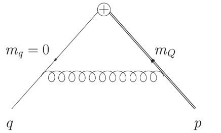
Figure 1: One-loop diagrams for the vertex functions. $q$ denotes the outgoing momentum and $p$ denotes the incoming momentum.

Figure 2: The $m_{Q}^{(0)}$ dependence of $\Delta_{\gamma_{k}}$ (circles) and $\Delta_{\gamma_{0}}$ (triangles) with the plaquette, the Iwasaki and the DBW2 gauge actions from top to bottom.

Figure 3: The same figure as Fig.  Perturbative determination of mass dependent renormalization and improvement coefficients for the heavy-light vector and axial-vector currents with relativistic heavy and domain-wall light quarks but for $c_{V_{k}}^{+}$ (circles) and $c_{V_{0}}^{+}$ (triangles).

Figure 4: The same figure as Fig.  Perturbative determination of mass dependent renormalization and improvement coefficients for the heavy-light vector and axial-vector currents with relativistic heavy and domain-wall light quarks but for $c_{V_{k}}^{-}$ (circles) and $c_{V_{0}}^{-}$ (triangles).

Figure 5: The same figure as Fig.  Perturbative determination of mass dependent renormalization and improvement coefficients for the heavy-light vector and axial-vector currents with relativistic heavy and domain-wall light quarks but for $c_{V_{k}}^{H}$ (circles) and $c_{V_{k}}^{L}$ (triangles).

Figure 6: The $m_{Q}^{(0)}$ dependence of $\Delta_{V_{0}}$, $\Delta_{V_{0}}^{\rm MF}$ and $\Delta_{V_{0}}^{\rm QNP+MF}$ with the plaquette, Iwasaki and DBW2 gauge action from top to bottom.

References

- (1) N. Yamada, Nucl. Phys. Proc. Suppl. 119, 93 (2003) [arXiv:hep-lat/0210035].
- (2) A. S. Kronfeld, Nucl. Phys. Proc. Suppl. 129, 46 (2004) [arXiv:hep-lat/0310063].
- (3) S. Aoki et al. [JLQCD Collaboration], Phys. Rev. Lett. 91, 212001 (2003) [arXiv:hep-ph/0307039].
- (4) S. Aoki et al. [JLQCD Collaboration], Nucl. Phys. Proc. Suppl. 106, 224 (2002) [arXiv:hep-lat/0110179].
- (5) N. Yamada et al. [JLQCD Collaboration], Nucl. Phys. Proc. Suppl. 106, 397 (2002) [arXiv:hep-lat/0110087].
- (6) S. Aoki, Y. Kuramashi and S.-I. Tominaga, Prog. Theor. Phys. 109, 383 (2003) [arXiv:hep-lat/0107009].
- (7) D. B. Kaplan, Phys. Lett. B 288 (1992) 342 [arXiv:hep-lat/9206013].
- (8) Y. Shamir, Nucl. Phys. B 406 (1993) 90 [arXiv:hep-lat/9303005].
- (9) V. Furman and Y. Shamir, Nucl. Phys. B 439 (1995) 54 [arXiv:hep-lat/9405004].
- (10) M. Luscher and P. Weisz, Commun. Math. Phys. 97, 59 (1985) [Erratum-ibid. 98, 433 (1985)].
- (11) A. X. El-Khadra, A. S. Kronfeld and P. B. Mackenzie, Phys. Rev. D 55, 3933 (1997) [arXiv:hep-lat/9604004].
- (12) S. Aoki, Y. Kayaba and Y. Kuramashi, arXiv:hep-lat/0309161.
- (13) Y. Iwasaki, UTHEP-118.
- (14) T. Takaishi, Phys. Rev. D 54, 1050 (1996).
- (15) P. de Forcrand et al. [QCD-TARO Collaboration], Nucl. Phys. B 577, 263 (2000) [arXiv:hep-lat/9911033].
- (16) S. Aoki, Y. Kayaba and Y. Kuramashi, Nucl. Phys. B 689, 127 (2004) [arXiv:hep-lat/0401030].
- (17) B. Sheikholeslami and R. Wohlert, Nucl. Phys. B 259, 572 (1985).
- (18) S. Aoki, T. Izubuchi, Y. Kuramashi and Y. Taniguchi, Phys. Rev. D 67, 094502 (2003) [arXiv:hep-lat/0206013]; ibid. 59, 094505 (1999) [arXiv:hep-lat/9810020].
- (19) D. Becirevic and J. Reyes, Nucl. Phys. Proc. Suppl. 129, 435 (2004) [arXiv:hep-lat/0309131].
- (20) E. Gulez, J. Shigemitsu and M. Wingate, Phys. Rev. D 69, 074501 (2004) [arXiv:hep-lat/0312017].
- (21) S. Kawabata, Comput. Phys. Commun. 41, 127 (1986); ibid. 88, 309 (1995).
- (22) G. P. Lepage and P. B. Mackenzie, Phys. Rev. D 48, 2250 (1993) [arXiv:hep-lat/9209022].
- (23) J. Harada, S. Hashimoto, K. I. Ishikawa, A. S. Kronfeld, T. Onogi and N. Yamada, Phys. Rev. D 65, 094513 (2002) [arXiv:hep-lat/0112044].
- (24) N. Kitazawa and T. Kurimoto, Phys. Lett. B 323, 65 (1994) [arXiv:hep-ph/9312225].