Light pseudoscalar decay constants, quark masses, and low energy constants from three-flavor lattice QCD

Abstract

As part of our program of lattice simulations of three flavor QCD with improved staggered quarks, we have calculated pseudoscalar meson masses and decay constants for a range of valence quark masses and sea quark masses on lattices with lattice spacings of about 0.125 fm and 0.09 fm. We fit the lattice data to forms computed with “staggered chiral perturbation theory.” Our results provide a sensitive test of the lattice simulations, and especially of the chiral behavior, including the effects of chiral logarithms. We find: $f_{\pi}=129.5\pm 0.9\pm 3.5\;{\rm Me\!V}$, $f_{K}=156.6\pm 1.0\pm 3.6\;{\rm Me\!V}$, and $f_{K}/f_{\pi}=1.210(4)(13)$, where the errors are statistical and systematic. Following a recent paper by Marciano, our value of $f_{K}/f_{\pi}$ implies $|V_{us}|=0.2219(26)$. Further, we obtain $m_{u}/m_{d}=0.43(0)(1)(8)$, where the errors are from statistics, simulation systematics, and electromagnetic effects, respectively. The partially quenched data can also be used to determine several of the constants of the low energy chiral effective Lagrangian: in particular we find $2L_{8}-L_{5}=-0.2(1)(2)\;\times 10^{-3}$ at chiral scale $m_{\eta}$, where the errors are statistical and systematic. This provides an alternative (though not independent) way of estimating $m_{u}$; the value of $2L_{8}-L_{5}$ is far outside the range that would allow the up quark to be massless. Results for $m_{s}^{\text{$\overline{\text{MS}}$}}$, $\hat{m}^{\text{$\overline{\text{MS}}$}}$, and $m_{s}/\hat{m}$ can be obtained from the same lattice data and chiral fits, and have been presented previously in joint work with the HPQCD and UKQCD collaborations. Using the perturbative mass renormalization reported in that work, we obtain $m_{u}^{\text{$\overline{\text{MS}}$}}=1.7(0)(1)(2)(2)\;{\rm Me\!V}$ and $m_{d}^{\text{$\overline{\text{MS}}$}}=3.9(0)(1)(4)(2)\;{\rm Me\!V}$ at scale $2\;{\rm Ge\!V}$, with errors from statistics, simulation, perturbation theory, and electromagnetic effects, respectively.

I INTRODUCTION

Using lattice QCD techniques, the masses and decay constants of light pseudoscalar mesons can be determined with high precision at fixed quark mass and lattice spacing. Assuming that the chiral and continuum extrapolations are under control, one can therefore calculate from first principles a number of physically important quantities, including

• Pion and kaon leptonic decay constants, $f_{\pi}$ and $f_{K}$, and their ratio.

• Low energy (“Gasser-Leutwyler” GASSER_LEUTWYLER ) constants $L_{i}$, in particular $L_{5}$, $L_{4}$, and the combinations $2L_{8}-L_{5}$ and $2L_{6}-L_{4}$.

• Quark mass ratios, such as $m_{s}/\hat{m}$, where $\hat{m}$ is the average of the $u$ and $d$ quark masses, and $m_{u}/m_{d}$.

• Absolute quark mass values, if the mass renormalization constant is known perturbatively or nonperturbatively.

The comparison of $f_{\pi}$ and $f_{K}$ with experiment provides a sensitive test of lattice methods and algorithms. A precise determination of $f_{K}$, or $f_{K}/f_{\pi}$ may in fact be turned around to determine the magnitude of the CKM element $V_{us}$, as emphasized recently by Marciano Marciano:2004uf . The quark masses are fundamental parameters of the Standard Model, and hence are phenomenologically and intrinsically interesting. Of special importance here is the up quark mass: if $m_{u}$ or $m_{u}/m_{d}$ can be bounded away from zero with small enough errors, it can rule out $m_{u}=0$ as a solution to the strong CP problem STRONG_CP ; Kaplan:1986ru . Finally, the Gasser-Leutwyler parameters give a concise summary of the properties of low energy QCD. In particular the combination $2L_{8}-L_{5}$ provides an alternative (although not independent) handle on the up quark mass COHEN ; Nelson:tb .

Extracting these important quantities is predicated on being able to control the chiral and continuum extrapolations. The improved staggered (Kogut-Susskind, KS) quarks IMP_ACTION ; SYM_GAUGE used here have the advantage in this respect of allowing us to simulate at quite small quark mass: Our lowest $m_{\pi}/m_{\rho}$ value is $\approx 0.3$, a pion mass of roughly $250\,{\rm Me\!V}$. On the other hand, these extrapolations are complicated by the fact that a single staggered quark field describes four species of quarks. We call this degree of freedom “taste” to distinguish it from physical flavor. We simulate the latter by introducing distinct staggered fields for each nondegenerate quark flavor; while we handle the former by taking the fourth root of the staggered quark determinant.

The fact that taste symmetry is violated at finite lattice spacing leads to both practical and theoretical complications. The improvement of the fermion action IMP_ACTION reduces the splittings among pseudoscalar mesons of various tastes to ${\cal O}(\alpha_{S}^{2}a^{2})$; yet the splittings are still numerically large, especially on our coarser lattices. This practical problem makes it impossible to fit our data with continuum chiral perturbation theory ($\chi$PT) expressions (see Refs. MILC_SPECTRUM and Aubin:2003ne , as well as discussion in Sec. IX.4). Instead, we must use “staggered chiral perturbation theory” (S$\chi$PT) LEE_SHARPE ; CB_FSB ; CA_CB1 ; CA_CB2 , which includes discretization effects within the chiral expansion. Using S$\chi$PT, we can take the chiral and continuum limits at the same time, and arrive at physical results with rather small systematic errors.

Theoretically, it is not obvious that, in the presence of taste-violations, the fourth root procedure commutes with the limit of lattice spacing $a\to 0$. Assuming that perturbation theory for the standard KS theory without the fourth root correctly reproduces a continuum four-taste theory, then the fourth root trick is correct in perturbation theory CB_MG_PQCHPT , since it just multiplies each virtual quark loop by $1/4$. However, nonperturbatively, the fourth root version is almost certainly not ultra-local at finite lattice spacing, and the possibility remains that it violates locality (and therefore universality) in the continuum limit. We believe that existing checks BIG_PRL ; GOTTLIEB_LAT03 ; MILC_SPECTRUM2 ; MASON_ALPHA of the formalism against experimental results already make this possibility unlikely. The current work adds more evidence that the method gives results that agree well with experiment and have the proper chiral behavior, up to controlled taste-violating effects that vanish in the continuum limit. However the question is not yet settled. We discuss this further in Sec. IX.4.7 and briefly refer to other recent work that addresses the issue.

This violation of taste symmetry arises because the full axial symmetry (at $m_{q}=0$) is broken to a single U(1) subgroup on the lattice. This means that only one of the pseudoscalars, which we call the “Goldstone meson”, has its mass and decay constant protected from renormalization. A study of pion masses and decay constants by the JLQCD collaboration JLQCD_FPI explored the masses and decay constants of all of the pseudoscalars in a quenched calculation. We concentrate almost exclusively here on Goldstone mesons, thus avoiding the necessity for renormalization.

We have generated a large “partially quenched” data set of Goldstone meson masses and decay constants using three flavors of improved KS sea quarks. These quantities have been computed with a wide range of sea quark masses (with $m_{u}=m_{d}\not=m_{s}$), and on lattices with lattice spacings of about 0.125 fm and 0.09 fm. We have 8 or 9 different valence quark masses available for each set of sea quark masses and lattice spacing. This data may be fit to chiral-logarithm forms from S$\chi$PT, which at present have been computed for Goldstone mesons only CA_CB1 ; CA_CB2 . However, since the masses for mesons of other tastes enter into the one-loop chiral logarithms of the Goldstone mesons, some control over those masses is also needed. We have computed most non-Goldstone “full QCD” (valence masses equal to sea masses) pion masses on most of our lattices. We can fit that data to the tree-level (LO) S$\chi$PT form, and use the results for splitting and slopes as input to the NLO terms for the Goldstone mesons. There is, of course, a NNLO error in this procedure, which we estimate in Sec. VI.2.

The outline of the rest of this paper is as follows: Section II explains the methodology used to compute raw lattice results (at fixed $a$ and fixed quark mass). In Sec. III, we describe the details of our simulations. We present a first look at the raw data in Sec. IV. Taste violations are discussed in Sec. V, followed in Sec. VI by a detailed description of our S$\chi$PT fitting forms. Relevant results from weak coupling perturbation theory are collected in Sec. VII. At the current level of precision, electromagnetic and isospin-violating effects cannot be ignored, and we discuss the necessary corrections and the attendant systematic errors in Sec. VIII. Section IX then presents the S$\chi$PT fits, including a description of fit ranges (in quark mass), an inventory of all fit parameters, the resulting fits, and a discussion of various issues relevant to the extraction of physical results. The discussion includes details of the continuum extrapolation, the evidence for chiral logarithms, an estimate of the systematic errors associated with using a (slightly) mass-dependent renormalization scheme, a critical look at the applicability and convergence of the chiral perturbation theory on our data set, bounds on residual finite volume effects, and some comments relevant to the fourth-root trick. In Sec. X, we present our final results, tabulate the systematic errors, and discuss prospects for improving the current determinations.

In collaboration with the HPQCD and UKQCD groups, we have previously reported results for $m_{s}^{\text{$\overline{\text{MS}}$}}$, the average $u$-$d$ quark mass $\hat{m}^{\text{$\overline{\text{MS}}$}}$, and $m_{s}/\hat{m}$ strange-mass . The data sets and chiral fits described in detail here are the same ones that were used in Ref. strange-mass .

II METHODOLOGY

For the axial current corresponding to the unbroken (except by quark mass) axial symmetry, the decay constant $f_{PS}$ can be found from the matrix element of $\bar{\psi}\gamma_{5}\psi$ between the vacuum and the pseudoscalar meson. In terms of the one component staggered fermion field $\bar{\psi}\gamma_{5}\psi$ corresponds to the operator

$${\cal O}_{P}(t)=\bar{\chi}^{a}(\vec{x},t)(-1)^{\vec{x}+t}\chi^{a}(\vec{x},t)\ .$$ (1)

Here $a$ is a summed color index. The relevant matrix element can be obtained from a pseudoscalar propagator using ${\cal O}_{P}$ as both the source and sink operator:

$$P_{PP}(t)=\frac{1}{V_{s}}\sum_{\vec{y}}\langle{\cal O}_{P}(\vec{x},0){\cal O}_{P}(\vec{y},t)\rangle=C_{PP}e^{-m_{PS}t}+{\rm excited\ state\ contributions}\ \ ,$$ (2)

where $m_{PS}$ is the mass of the pseudoscalar, and $V_{s}$ is the spatial volume.

The decay constant is obtained from $C_{PP}$ by JLQCD_FPI ; TOOLKIT

$$f_{PS}=(m_{x}+m_{y})\sqrt{\frac{V_{s}}{4}}\sqrt{\frac{C_{PP}}{m_{PS}^{3}}}\ ,$$ (3)

where $m_{x}$ and $m_{y}$ are the two valence quark masses in the pseudoscalar meson. Throughout this paper we use the convention where the experimental value of $f_{\pi}$ is approximately $131\;{\rm Me\!V}$. Note that in computing this meson propagator we must take care to normalize the lattice Dirac matrix as $M=am+{D\!\!\!\!/}$. The four in the denominator arises from the number of tastes natural to the Kogut-Susskind formulation. (See unnumbered equations between Eqs. 7.2 and 7.3 in Ref. TOOLKIT .)

However, the point operator ${\cal O}_{P}$ has large overlap with excited states. For calculating masses it is customary to use an extended source operator that suppresses these overlaps, together with a point sink. In our case, this extended operator is a “Coulomb wall,” i.e., we fix to the lattice Coulomb gauge and sum over all lattice points on a timeslice:

$${\cal O}_{W}(t)=\sum_{\vec{x},\vec{y}}\bar{\chi}(\vec{x},t)(-1)^{\vec{x}+t}\chi(\vec{y},t)\ \ \ .$$ (4)

We can calculate propagators with any source or sink operator we wish. Ignoring excited state contributions, we have for example

$$\langle{\cal O}_{P}(\vec{x},0){\cal O}_{W}(t)\rangle=C_{PW}e^{-m_{\pi}t}\ \ \ .$$ (5)

We will use the shorthand “PP” for point-source point-sink propagators, “WP” for Coulomb-wall-source point-sink propagators, “PW” for point-source Coulomb-wall-sink propagators, and “WW” for Coulomb-wall source and sink propagators. In previous calculations of pseudoscalar decay constants the relation $C_{PP}=C_{WP}^{2}/C_{WW}$ has often been used to get the point-point amplitude. However, the wall-wall propagator has large statistical fluctuations and severe problems with excited states, as was discussed in Ref. JLQCD_FPI . To be able to use the PP operator to get $C_{PP}$ directly, rather than indirectly by way of the ratio formula, one needs much better statistics. We do this by replacing the point source with a “random-wall” source, which simulates many point sources. We set the source on each site of a time slice to a three component complex unit vector with a random direction in color space, and use this as the source for a conjugate gradient inversion to compute the quark propagator, whose magnitude is squared to produce the Goldstone pion propagator. Thus, contributions to a meson propagator where the quark and antiquark originate on different spatial sites will average to zero and, after dividing by the spatial lattice volume, this source can be used instead of ${\cal O}_{P}$.

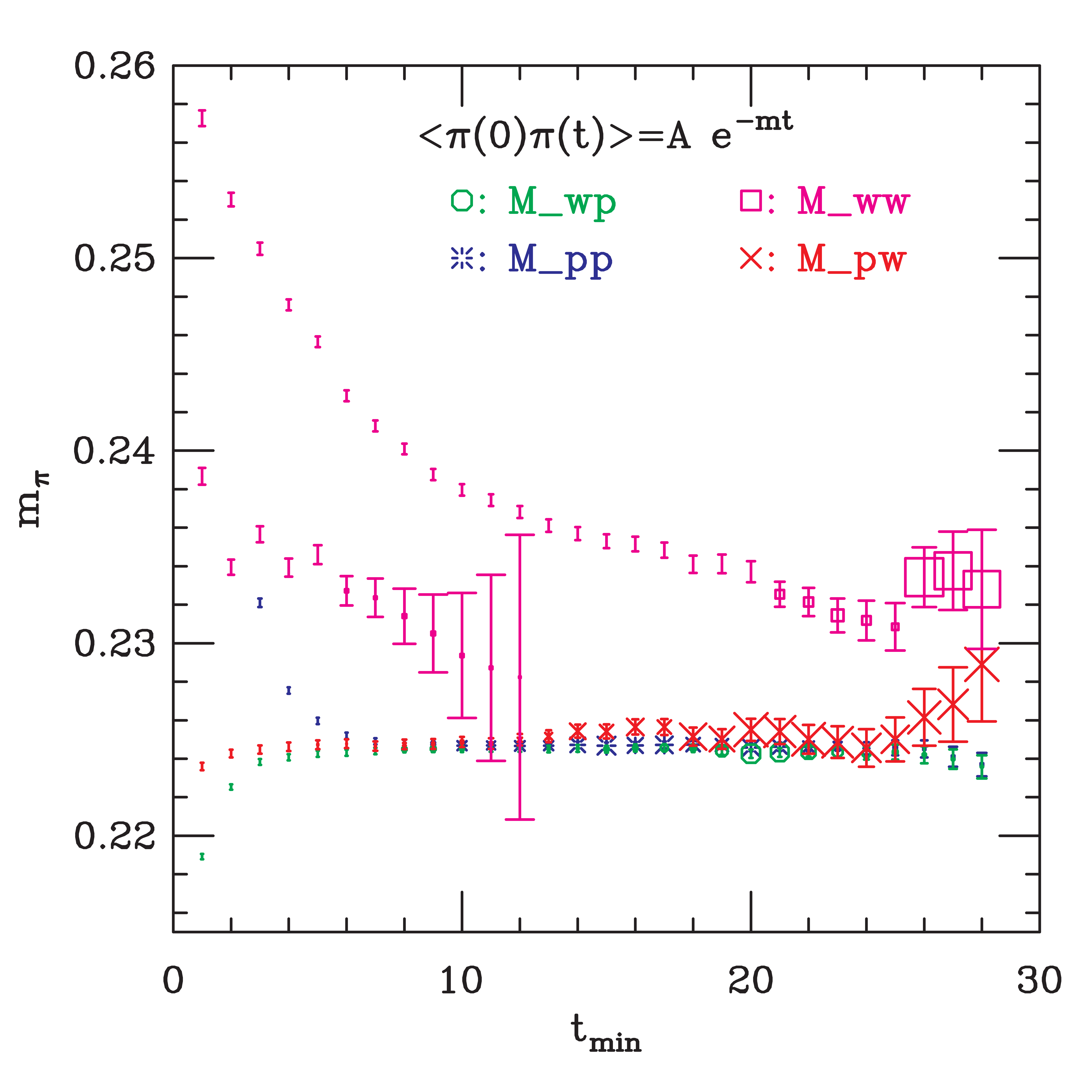
Figure 1: Pion masses with random-wall and Coulomb-wall sources and point and Coulomb-wall sinks from the coarse set with sea quark lattice masses 0.01,0.05 (see Table 1). The red crosses are random-wall source and Coulomb-wall sink, and the green octagons are Coulomb-wall source and point sink (summed over spatial sites to project out the zero momentum states). The blue bursts are from a random-wall source and point sink, and the magenta squares have a Coulomb-wall source and sink. The lower set of “WW” points include an excited state in the fit. The symbol size is proportional to the confidence level of the fit, with the symbol size in the labels corresponding to 50%.

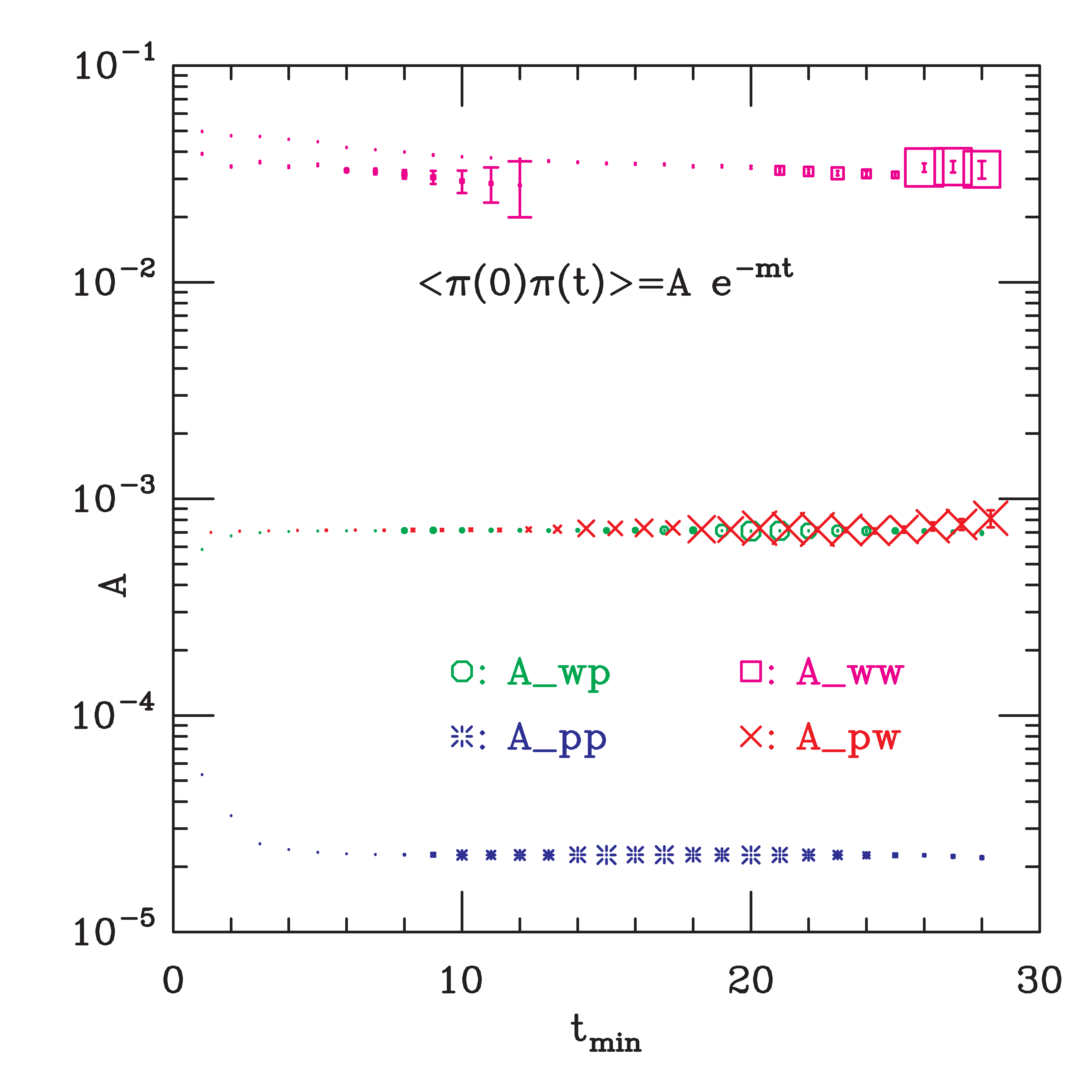
Figure 2: Same as Fig. 1 but for pion propagator amplitudes. The lower set of “WW” points again include an excited state in the fit. The “PW” symbols have been displaced slightly to the right to separate them from the “WP” points.

Figures 1 and 2 show masses and amplitudes from pion propagators with random-wall and Coulomb-wall sources and sinks. In Fig. 1, we can see that extraction of masses from the “WW” propagators is almost hopeless. Including an excited state helps, but statistical errors become very large. In Fig. 2, the WW amplitudes are also slower to plateau, though not as bad as the masses. As a consistency check, note that the WP and PW amplitudes are equal, and the masses extracted from the diagonal PP and WW propagators approach their value from above (since excited states must contribute to these propagators with the same sign as the ground state). As an additional illustration of the difficulties with using the Coulomb-wall—Coulomb-wall propagator, Fig. 3 plots the ratio of the point-point pion propagator (using the random wall source) to the alternative $P_{PW}P_{WP}/P_{WW}$ (with a different mass than in Figs. 1 and 2). While this ratio is approaching one, it is clear that we would either need very large minimum time in the fit or a careful removal of excited states to use the “WW” propagators.

Given the problems with the WW propagators, we have opted to use only the Coulomb-wall—point-sink and random-wall—point-sink propagators. We performed a simultaneous fit to these two propagators, with an amplitude for each propagator and a common mass. In these fits the WP propagator dominates the determination of the mass; while the amplitude of the PP propagator is required for computing the decay constant. Since the combination $C_{PP}/m_{\pi}^{3}$ is needed for determining $f_{\pi}$ and the mass and amplitude in a fit to a meson propagator are strongly correlated, we used this combination as one of our fitting parameters. That is, we fit the point—point and wall—point meson correlators to

$$P_{PP} = m_{\pi}^{3}\,A_{PP}e^{-m_{\pi}t}$$

$$P_{WP} = m_{\pi}^{3}\,A_{WP}e^{-m_{\pi}t}$$ (6)

so that $A_{PP}$ is the desired combination $C_{PP}/m_{\pi}^{3}$. Since the correlation between $m_{\pi}$ and the propagator amplitude is positive, the statistical error on the quantity $C_{PP}/m_{\pi}^{3}$ is somewhat smaller than a naive combination of the errors on $C_{PP}$ and $m_{\pi}$.

III SIMULATIONS

These calculations were made on lattices generated with a one loop Symanzik and tadpole improved gauge actionSYM_GAUGE ; LEPAGE_MACKENZIE and an order $a^{2}$ tadpole improved Kogut-Susskind quark action IMP_ACTION . Parameters of most of the lattices, as well as the light hadron spectrum, are in Ref. MILC_SPECTRUM ; MILC_SPECTRUM2 . The determination of the static quark potential, used here to set the lattice spacing, is presented in Ref. MILC_SPECTRUM ; MILC_SPECTRUM2 ; MILC_POTENTIAL . In addition to the runs tabulated in Ref. MILC_SPECTRUM , we now have a partially completed run with $a\hat{m}^{\prime}=0.005$ and $am^{\prime}_{s}=0.05$. (Here and below, the primes on masses indicate that they are the dynamical quark masses used in the simulations, not the physical masses $\hat{m}$ and $m_{s}$.) In addition, we have results from two runs at a finer lattice spacing, $a\approx 0.09$ fm, with quark masses of $a\hat{m}^{\prime},am^{\prime}_{s}=0.0124,0.031$ and $0.0062,0.031$. These runs, with $\hat{m}^{\prime}=0.4m^{\prime}_{s}$ and $0.2m^{\prime}_{s}$, are analogous to the coarse lattice runs with $a\hat{m}^{\prime},am^{\prime}_{s}=0.02,0.05$ and $0.01,0.05$ respectively. All of these lattices have a spatial size of about 2.5 fm with the exception of the $a\hat{m}^{\prime},am^{\prime}_{s}=0.005,0.05$ run, where the spatial size is about 3.0 fm. Table 1 lists the parameters of the runs used here.

We note here that the values for $am^{\prime}_{s}$ were approximately tuned from the vector to pseudoscalar meson mass ratio in initial runs with fairly heavy quarks. Our best determinations of the physical strange quark mass at these lattice spacings turned out to be lower by 8 to 22% (coarse) and 6 to 12% (fine) than the nominal values $m^{\prime}_{s}$, where the range depends on whether or not taste-violating terms (as determined by S$\chi$PT fits) are set to zero before demanding that $m_{\pi}$ and $m_{K}$ take their physical values on a given lattice.

$a\hat{m}^{\prime}$ / $am^{\prime}_{s}$	$10/g^{2}$	dims.	lats.	$am_{\pi}$	$am_{K}$	$af_{\pi}$	$af_{K}$
0.03 / 0.05	6.81	$20^{3}\times 64$	262	0.37787(18)	0.43613(19)	0.11452(31)	0.12082(31)
0.02 / 0.05	6.79	$20^{3}\times 64$	485	0.31125(16)	0.40984(21)	0.10703(18)	0.11700(21)
0.01 / 0.05	6.76	$20^{3}\times 64$	608	0.22447(17)	0.38331(24)	0.09805(14)	0.11281(17)
0.007 / 0.05	6.76	$20^{3}\times 64$	447	0.18891(20)	0.37284(27)	0.09364(20)	0.11010(28)
0.005 / 0.05	6.76	$24^{3}\times 64$	137	0.15971(20)	0.36530(29)	0.09054(33)	0.10697(40)
0.0124 / 0.031	7.11	$28^{3}\times 96$	531	0.20635(18)	0.27217(21)	0.07218(16)	0.07855(17)
0.0062 / 0.031	7.09	$28^{3}\times 96$	583	0.14789(18)	0.25318(19)	0.06575(13)	0.07514(17)

Table 1: Parameters of the simulations in units of the lattice spacing. The first four columns are the dynamical quark masses $a\hat{m}^{\prime}/am^{\prime}_{s}$, the gauge coupling $10/g^{2}$, the lattice dimensions, and the number of configurations used in these calculations. The remaining four columns are the “diagonal” pseudoscalar masses and amplitudes, with valence quark masses equal to the sea quark masses. The masses shown here come from a separate spectrum calculation, using more source time slices than were used in the partially quenched calculations, and using more lattices at $a\hat{m}^{\prime}=0.03$. Equation 7 can be used to express these masses and decay constants in units of $r_{1}$.

Pseudoscalar propagators were calculated on lattices separated by six units of simulation time, using two source time slices per lattice. For the coarse lattices, nine valence quark masses were used, ranging from $0.1m^{\prime}_{s}$ to $m^{\prime}_{s}$; while for the fine lattices eight masses ranging from $0.14m^{\prime}_{s}$ to $m^{\prime}_{s}$ were used. In all but one of the runs, the source slices were taken at different points in successive lattices, which leads to smaller autocorrelations than using the same source time slices on all lattices. The effects of the remaining correlations among the sample lattices were estimated in two ways. First, jackknife error estimates for the masses and decay constants were made eliminating one lattice at a time, and again eliminating four successive lattices. Secondly, an integrated autocorrelation time was estimated by summing the autocorrelations of the single elimination jackknife results over separations from one to five samples (six to thirty simulation time units) $\tau_{int}=\sum_{1}^{5}2C_{i}$, where $C_{i}$ is the normalized autocorrelation of jackknife results omitting lattices separated by $6i$ time units. The error estimate including the effects of autocorrelations is a factor of $\sqrt{1+\tau_{int}}$ larger than the error from the single elimination jackknife fit. Table 2 summarizes the results of these tests. The numbers in Table 2 vary a lot, consistent with the well known difficulties in measuring autocorrelations on all but the longest runs. Since we actually expect the autocorrelations to be smooth functions of the quark mass, we account for them by increasing all the elements of the covariance matrix by an approximate average of these factors squared, $(1.10)^{2}$, which is equivalent to increasing error estimates by a factor of 1.10.

$a\hat{m}^{\prime}$ / $am^{\prime}_{s}$	$10/g^{2}$	$\frac{\Delta m^{2}(4)}{\Delta m^{2}(1)}$	$\frac{\Delta f(4)}{\Delta f(1)}$	$\tau_{int,m}$	$\tau_{int,f}$
0.03 / 0.05	6.81	1.10	1.16	0.25	0.15
0.02 / 0.05	6.79	1.07	1.00	0.01	-0.09
0.01 / 0.05	6.76	1.28	1.12	0.30	0.27
0.007 / 0.05	6.76	1.05	0.90	-0.02	-0.03
0.005 / 0.05	6.76	1.06	1.20	-0.04	-0.04
0.00124 / 0.031	7.11	1.10	1.13	0.25	0.15
0.00062 / 0.031	7.09	1.10	0.95	0.22	-0.01

Table 2: Estimates of the effects of autocorrelations. $\Delta m^{2}(4)/\Delta m^{2}(1)$ is the ratio of error estimates for the squared pion mass between jackknife estimates with a block size of four and a block size of one. $\Delta f^{2}(4)/\Delta f^{2}(1)$ is the same thing for the decay constant. $\tau_{int,m}$ and $\tau_{int,f}$ are the integrated autocorrelation times for the squared pion mass and decay constant. All of these numbers are averaged over the valence quark masses.

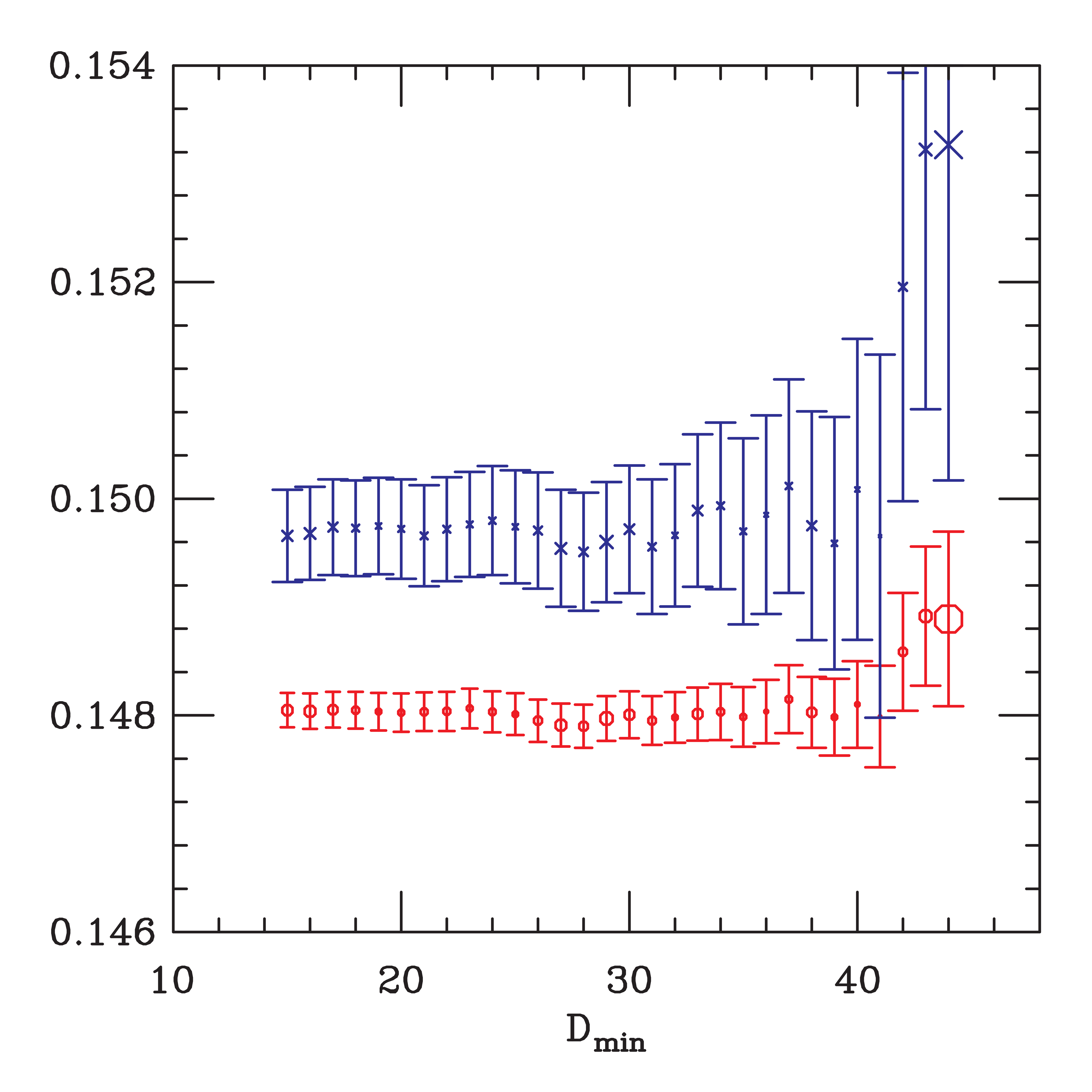
Figure 4: Pion masses (red octagons) and amplitudes (blue crosses) as a function of the minimum time distance in the fit, from the fine set with sea quark lattice masses 0.0062,0.031 (see Table 1). The amplitudes have been multiplied by 175.

Propagators were fit to Eq. II using a minimum time distance of $20a$ for the coarse lattices and $30a$ for the fine lattices. At these distances, the contamination from excited states is at most comparable to the statistical errors. For example, Fig. 4 shows results for pion masses and amplitudes as a function of minimum fitting distance for one of the fine runs. Since our other systematic errors are significantly larger than statistical errors (see Sec. X), we can neglect the systematic effect due to excited states.

For each run, the propagator fitting produced a pion mass and decay constant for each combination of valence quark masses. We call the two valence quarks in a particular meson $x$ and $y$; there are 45 different combinations of $m_{x}$,$m_{y}$ for the coarse lattices and 36 for the fine, although, as described in Sec. IX.1, the largest valence quark masses were not used in all of the fits. All of the masses and decay amplitudes from a single run are correlated. For each run with $N$ samples, a covariance matrix describing the fluctuations of all of these numbers was made by doing a single elimination jackknife fit, omitting one lattice at a time, and rescaling the covariance matrix of the jackknife fits by $(N-1)^{2}$. A single elimination jackknife, rather than one where larger blocks were omitted, was used because getting a reliable covariance matrix requires a number of samples large compared to the dimension of the matrix. Then, to account for autocorrelations, this covariance matrix was rescaled by the factor estimated above. Finally, to allow simultaneous fitting of the meson decay constants and masses from all of the runs as a function of valence and sea quark masses, the covariance matrices from the individual runs were combined into a large block-diagonal covariance matrix. (Runs with different sea quark masses or gauge couplings are independent, so correlations between different runs can be set to zero.)

Fitting the pseudoscalar propagators produces masses and decay constants in units of the lattice spacing $a$, and to convert to physical units we must estimate $a$ from a calculation of some dimensional quantity whose value is known. This amounts to saying that we are calculating ratios of these quantities to some other quantity calculated from these simulations. We express our results in units of a length obtained from the static quark potential, $r_{1}$, where $r_{1}^{2}\,F(r_{1})=1.0$ SOMMER ; MILC_POTENTIAL . This has the advantage that $r_{1}$ can be accurately determined in units of the lattice spacing. But $r_{1}$ is not a directly measurable quantity, and its physical value must in turn be obtained from some other quantities. We have calculated the static quark potential in all of these runs, and fit it to determine $r_{1}/a$. To smooth out statistical fluctuations in these values, we then computed a “smoothed $r_{1}$” by fitting the $r_{1}/a$ values to a smooth function. A simple form, which gives a good fit over the range of quark masses and gauge coupling used here, is MILC_SPECTRUM2

$$\log(r_{1}/a)=C_{00}+C_{10}(10/g^{2}-7)+C_{01}am_{tot}+C_{20}(10/g^{2}-7)^{2}\ ,$$ (7)

where $m_{tot}=2\hat{m}^{\prime}+m^{\prime}_{s}$. The results of the fit are

$$C_{00}=1.258(3) C_{10}=0.937(9)$$

$$C_{01}=-0.83(3) C_{20}=-0.27(2)$$ (8)

When we need an absolute lattice scale, we start with the scale from $\Upsilon$ $2S$-$1S$ or $1P$-$1S$ splittings, determined by the HPQCD group BIG_PRL ; HPQCD_PRIVATE . This gives a scale $a^{-1}=1.588(19)$ GeV on the coarse $0.01/0.05$ lattices, and $a^{-1}=2.271(28)$ GeV on the fine $0.0062/0.031$ lattices. For light quark masses $\raise 1.29167pt\hbox{$<$\kern-7.5pt\lower 4.30554pt\hbox{$\sim$}}m_{s}/2$, the mass dependence of these quantities and of $r_{1}$ appears to be slight, and we neglect it. With our smoothed values of $r_{1}/a$, we then get $r_{1}=0.324(4)$ fm on the coarse lattices and $r_{1}=0.320(4)$ fm on the fine lattices.

To extrapolate $r_{1}$ to the continuum, we first assume that the dominant discretization errors go like $\alpha_{S}a^{2}$. Using $\alpha_{V}(q^{*})$ Davies:2002mv (with scale $q^{*}=\pi/a$) for $\alpha_{S}$ gives a ratio $(\alpha_{S}a^{2})_{\rm fine}/(\alpha_{S}a^{2})_{\rm coarse}=0.427$. Extrapolating away the discretization errors linearly then results in $r_{1}=0.317(7)$ fm in the continuum. However, taste-violating effects, while formally ${\cal O}(\alpha^{2}_{S}a^{2})$ and hence subleading, are known to be at least as important as the leading errors in some case. Therefore, one should check if the result changes when the errors are assumed to go like $\alpha^{2}_{S}a^{2}$. Taking $\alpha_{S}=\alpha_{V}(3.33/a)$ gives a ratio $(\alpha^{2}_{S}a^{2})_{\rm fine}/(\alpha^{2}_{S}a^{2})_{\rm coarse}=0.375$; while a direct lattice measurement of the taste-splittings gives a ratio of $0.35$. Extrapolating linearly to the continuum then implies $r_{1}=0.318(7)$ fm or $r_{1}=0.319(6)$ fm, respectively, in agreement with the previous result. For our final result, we use an “average” ratio of 0.4 and add the effect of varying this ratio in quadrature with the statistical error. We obtain $r_{1}=0.317(7)$ fm. A systematic error of $0.03$ fm in $r_{1}$ from our choice of fitting methods is omitted since it is common to all our runs and cancels out in the final results here. Using our current value $r_{0}/r_{1}=1.472(7)$, the result for $r_{1}$ implies $r_{0}$ is about 7% smaller than the standard phenomenological choice $r_{0}=0.5\;$fm, although the difference is within the expected range of error of the phenomenological estimates SOMMER .

IV First Look at Results

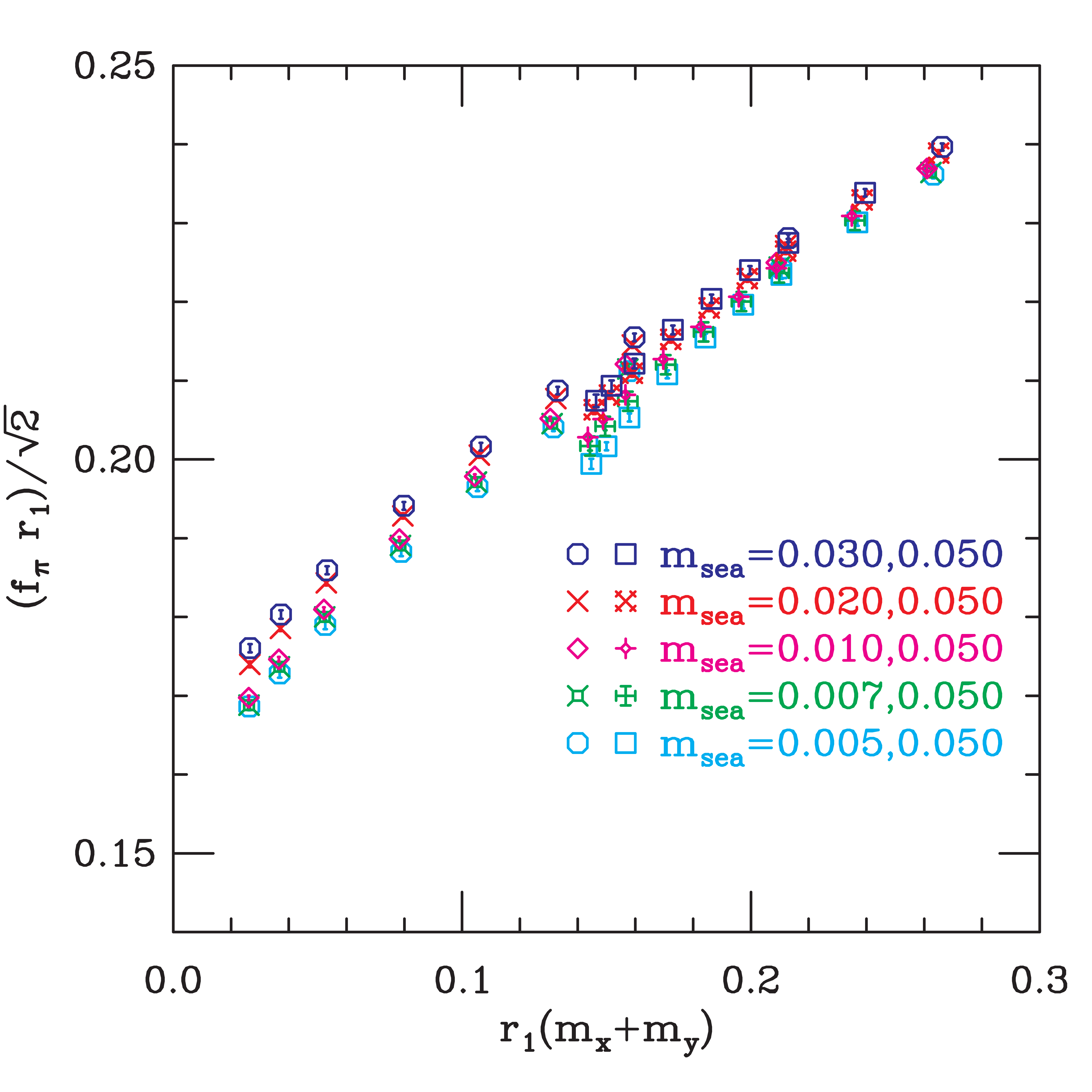
Figure 6: Decay constants in units of $r_{1}$ with $a\approx 0.125$ fm. The abscissa and symbols are the same as in Fig. 5.

Figures 5 and 6 present pseudoscalar masses and decay constants in units of $r_{1}$ as functions of the valence quark masses for several different light quark masses. All of these points are from the lattices with $a\approx 0.125$ fm. Figure 5 also contains pion masses where the sea quark mass varies along with the valence quark masses.

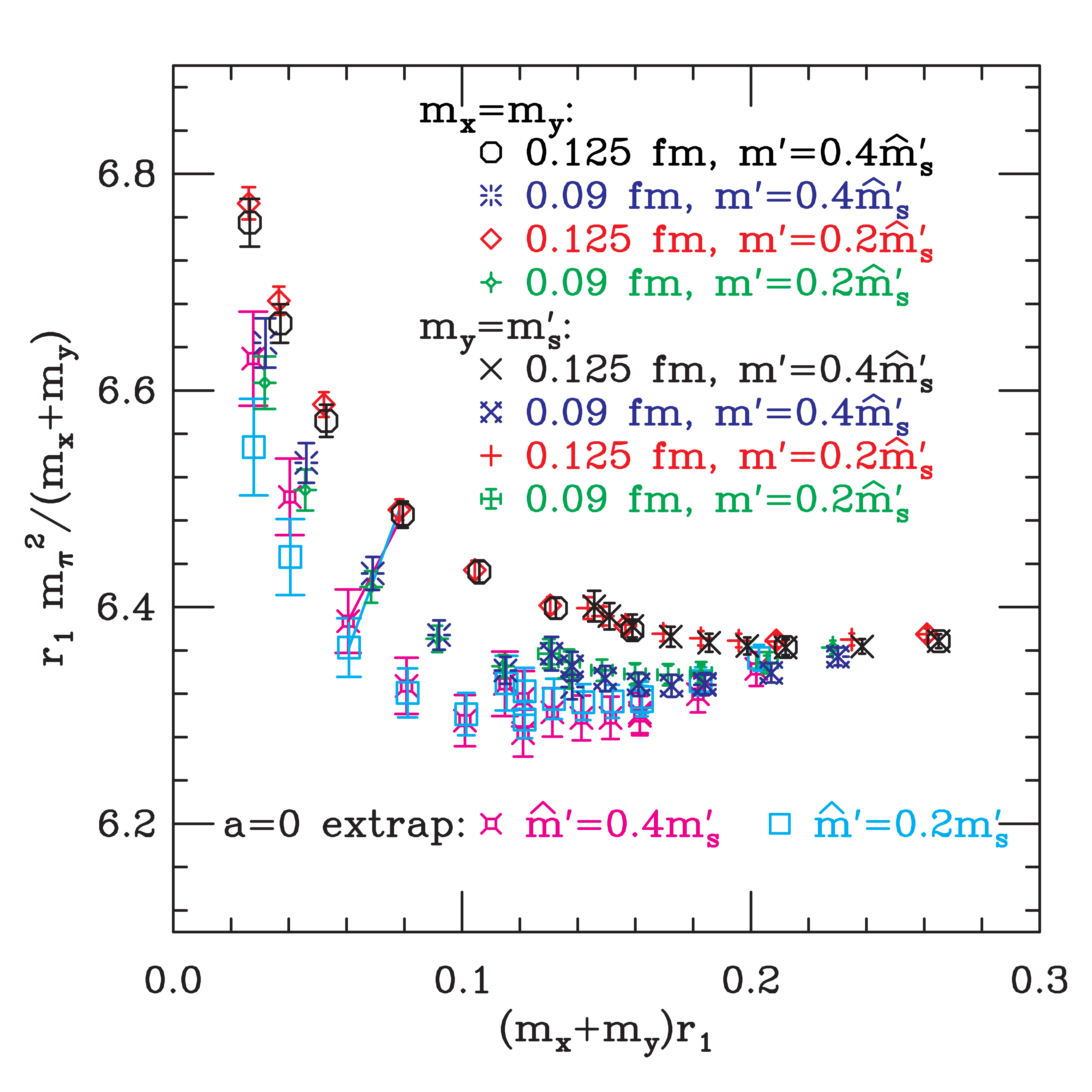
Figure 7: “Pion” masses ($m_{x}=m_{y}$) and “kaon” masses ($m_{y}=m^{\prime}_{s}$) with sea quark masses $\hat{m}^{\prime}=0.4m^{\prime}_{s}$ and $\hat{m}^{\prime}=0.2m^{\prime}_{s}$ at $a\approx 0.125$ fm and $a\approx 0.09$ fm. A “point by point” extrapolation to $a=0$ (fancy magenta squares: $\hat{m}^{\prime}=0.4m^{\prime}_{s}$, and cyan squares: $\hat{m}^{\prime}=0.2m^{\prime}_{s}$) is also included.

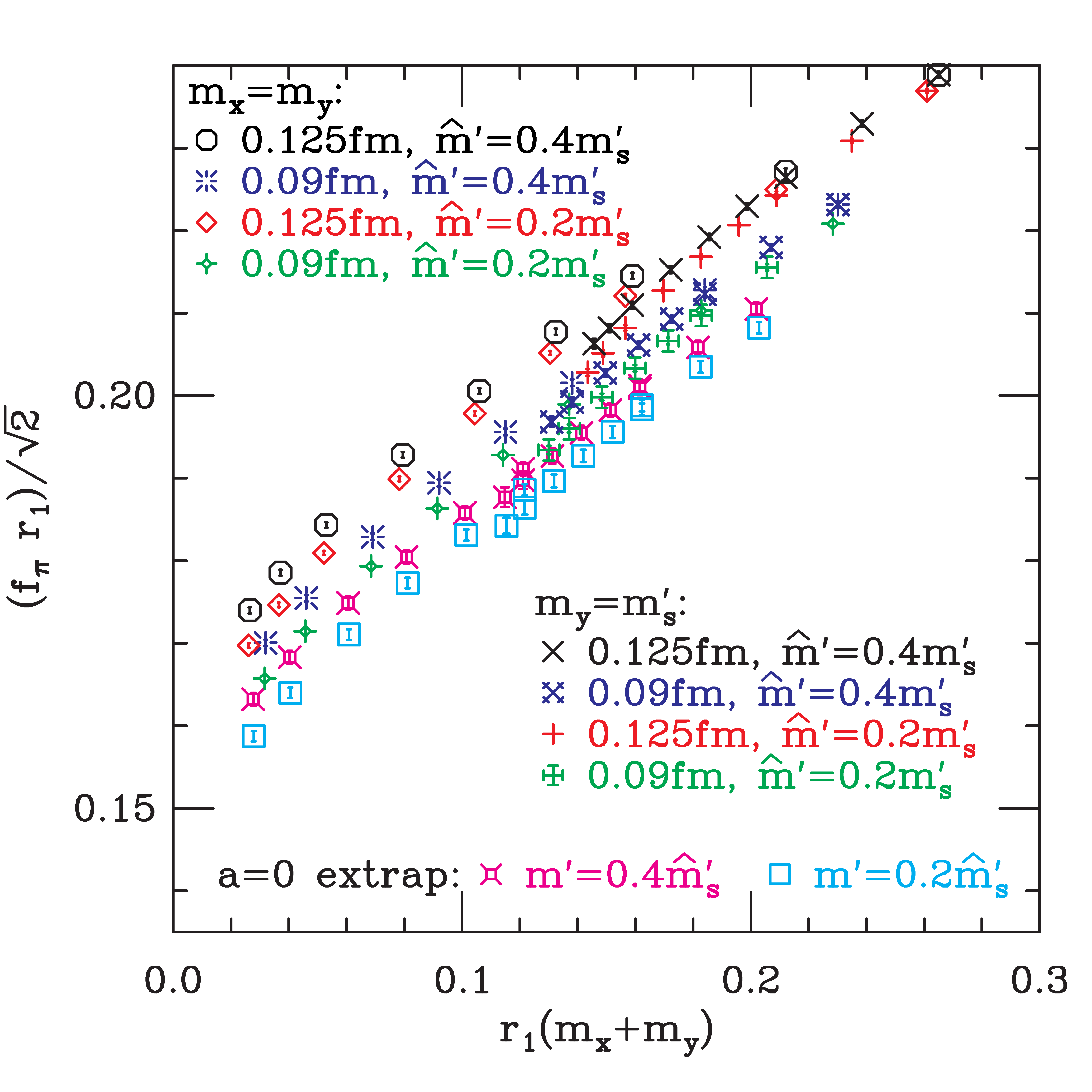
Figure 8: Same as Fig. 7 but for decay constants.

Figures 7 and 8 show the effect of changing the lattice spacing. For lattice spacings $a\approx 0.125$ fm and $a\approx 0.09$ fm we show results with $\hat{m}^{\prime}=0.4m^{\prime}_{s}$ and $\hat{m}^{\prime}=0.2m^{\prime}_{s}$, again in units of $r_{1}$. The horizontal axis is again the sum of the valence quark masses in the meson. These figures also show a crude extrapolation to $a=0$, made by taking a linear extrapolation in $\alpha_{S}a^{2}$ using pairs of points with the same $\hat{m}^{\prime}/m^{\prime}_{s}$. In Fig. 7 one pair of extrapolated points has diagonal lines showing the data points that were extrapolated to produce this point. In hindsight, $m^{\prime}_{s}$ used in the $a\approx 0.09$ fm runs was smaller than that used in the $a\approx 0.125$ fm runs, as indicated by the fact that the finer lattice points fall slightly to the left of the corresponding coarse lattice points.

V Taste symmetry violations

As mentioned above, we use the term “taste” to denote the different staggered-fermion species resulting from doubling. At finite lattice spacing, taste symmetry is violated. Although the improved staggered action reduces the taste violating effects to ${\cal O}(\alpha_{S}^{2}a^{2})$ from ${\cal O}(\alpha_{S}a^{2})$ with unimproved staggered fermions, the violations are still quite significant numerically.

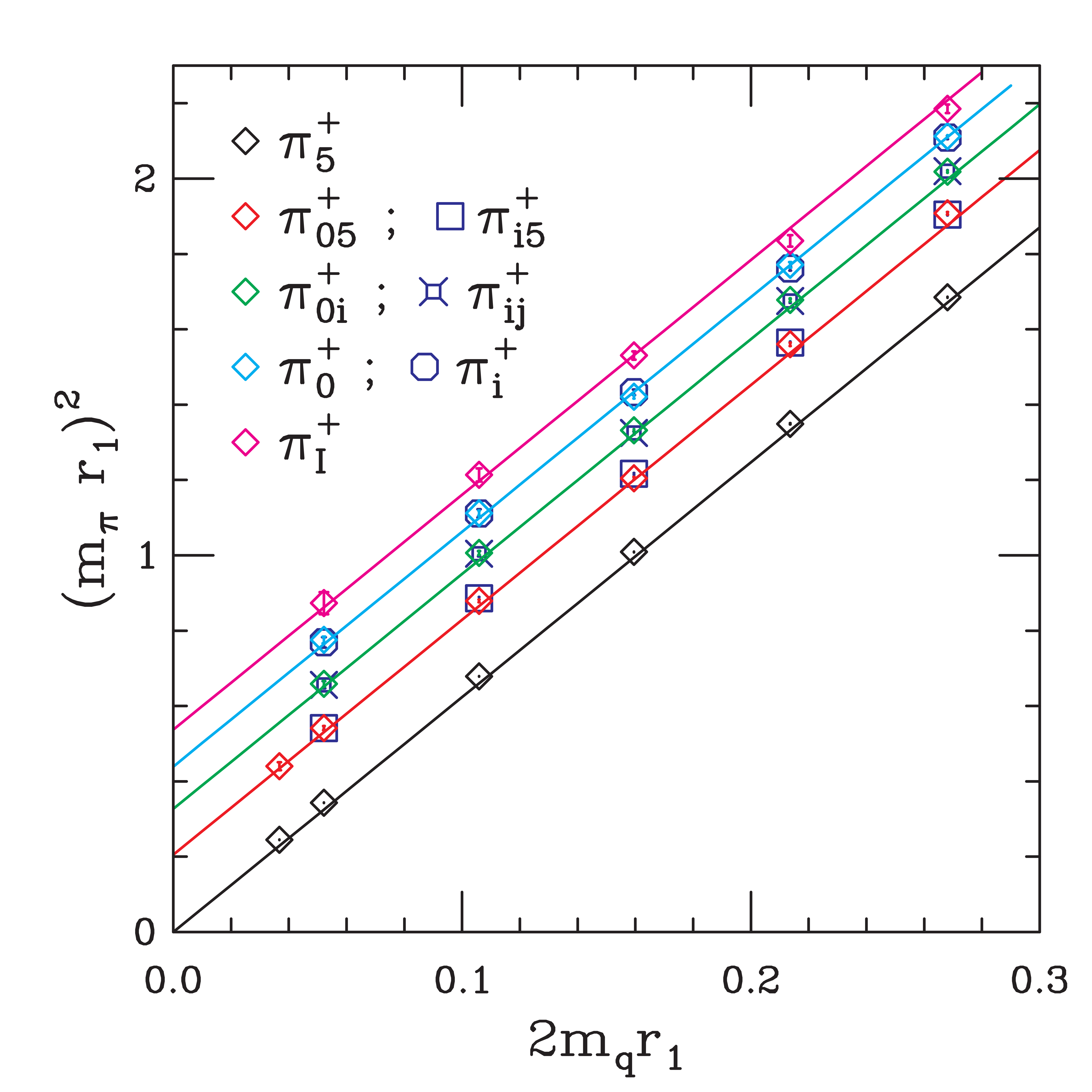
Figure 9: Squared masses of charged pions for various tastes on the coarse lattices. We use $r_{1}$ to set the scale. Tastes that are degenerate by $SO(4)$ symmetry are fit together.

Figure 9 shows the splittings between pions of various tastes on our coarse lattices. There are 16 such pions, $\pi_{B}$, where $B={5,\mu 5,\mu\nu,\mu,I}$ ($\nu>\mu$) labels taste matrices in the taste Clifford algebra generated by Euclidean gamma matrices $\xi_{\mu}$. The $\pi_{5}$ is the Goldstone (pseudoscalar taste) pion, whose mass is required to vanish in the chiral limit by the exact (non-singlet) lattice axial symmetry. All the pions in Fig. 9 are flavor-charged, i.e., $\pi^{+}$ mesons. Thus there are no contributions from disconnected graphs, even for the taste-singlet $\pi^{+}_{I}$. The approximate “accidental” $SO(4)$ identified by Lee and Sharpe LEE_SHARPE is clearly a good symmetry: there is near degeneracy between $\pi^{+}_{05}$ and $\pi^{+}_{i5}$, between $\pi^{+}_{0i}$ and $\pi^{+}_{ij}$, and between $\pi^{+}_{0}$ and $\pi^{+}_{i}$. When we assume such degeneracy, we can think of the index $B$ as running over the multiplets $5,A,T,V,I$ with degeneracies 1, 4, 6, 4, 1, respectively.

The fit in Fig. 9 is to the tree-level chiral form given in Refs. LEE_SHARPE ; CA_CB1 :

$$m^{2}_{\pi^{+}_{B}}=2\mu_{\rm tree}\hat{m}+a^{2}\Delta_{B}\ .$$ (9)

The slope, $\mu_{\rm tree}$, is the same for all tastes, but there are constant splittings for each non-Goldstone multiplet ($\Delta_{5}=0$). Although the fit is poor (chiral logs, including taste-violations, are needed), it does give the pion squared masses within a few per cent: The biggest deviation, 7%, is for the Goldstone pion at the lowest mass; most other deviations are $\sim\!2\%$.

Table 3 shows the values of $a^{2}\Delta_{B}$ coming from the fit on the coarse lattices. On the fine lattices, we have measured non-Goldstone pion masses only on the set with quark masses $0.0124$, $0.031$. So we directly compare the splittings with those of the corresponding coarse lattice (masses $0.02$, $0.05$). The fine-lattice splittings are smaller by a common factor of $0.35$, within errors. This is consistent with the expectation that taste violations go like ${\cal O}(\alpha^{2}_{S}a^{2})$. Indeed, if we take $\alpha_{S}=\alpha_{V}(q^{*})$ Davies:2002mv and choose $q^{*}=\pi/a$ because taste violations occur at the scale of the cutoff, we find

$$\frac{(\alpha^{2}_{V}(q^{*}\!\!=\!\pi/a)\;a^{2})_{\rm fine}}{(\alpha^{2}_{V}(q^{*}\!\!=\!\pi/a)\;a^{2})_{\rm coarse}}=0.372\ .$$ (10)

taste ($B$)	$r_{1}^{2}(a^{2}\Delta_{B})_{\rm coarse}$	$\frac{(a^{2}\Delta_{B})_{\rm fine}}{(a^{2}\Delta_{B})_{\rm coarse}}$
A	0.205(2)	0.344(23)
T	0.327(4)	0.353(18)
V	0.439(5)	0.347(22)
I	0.537(15)	0.384(33)

Table 3: Mass-squared splittings in units of $r_{1}$ for the coarse lattices, and the ratio of fine to coarse splittings. Results from tastes that are degenerate under the accidental $SO(4)$ have been combined.

The ratio of taste-violating terms between fine and coarse lattices is an input to the chiral fits for Goldstone pions discussed below. The measured splitting ratio of $0.35$ is used as a central value. The error can be estimated by varying $q^{*}$ in Eq. (10): $q^{*}=\pi/(2a)$ gives a ratio of $0.324$; while $2\pi/a$ gives $0.398$. We take $0.3$–$0.4$ as an appropriate range for our analysis of systematics.

We warn the reader here that the notation in Eq. (9) can be slightly misleading. We have shown explicitly the $a^{2}$ factor in the taste-violating splitting, $a^{2}\Delta_{B}$, but this does not mean that $\Delta_{B}$ itself is independent of lattice spacing, or even that it approaches a non-zero constant in the continuum limit. Indeed, the argument above implies that $\Delta_{B}$ is a slowly varying function of $a$ that goes like $\alpha_{V}^{2}(\pi/a)$ for small $a$. A similar comment applies to the other taste-violating parameters introduced in Sec. VI.1: the $a^{2}$ dependence is always shown explicitly, but dependence on $a$ through the coupling is hidden.

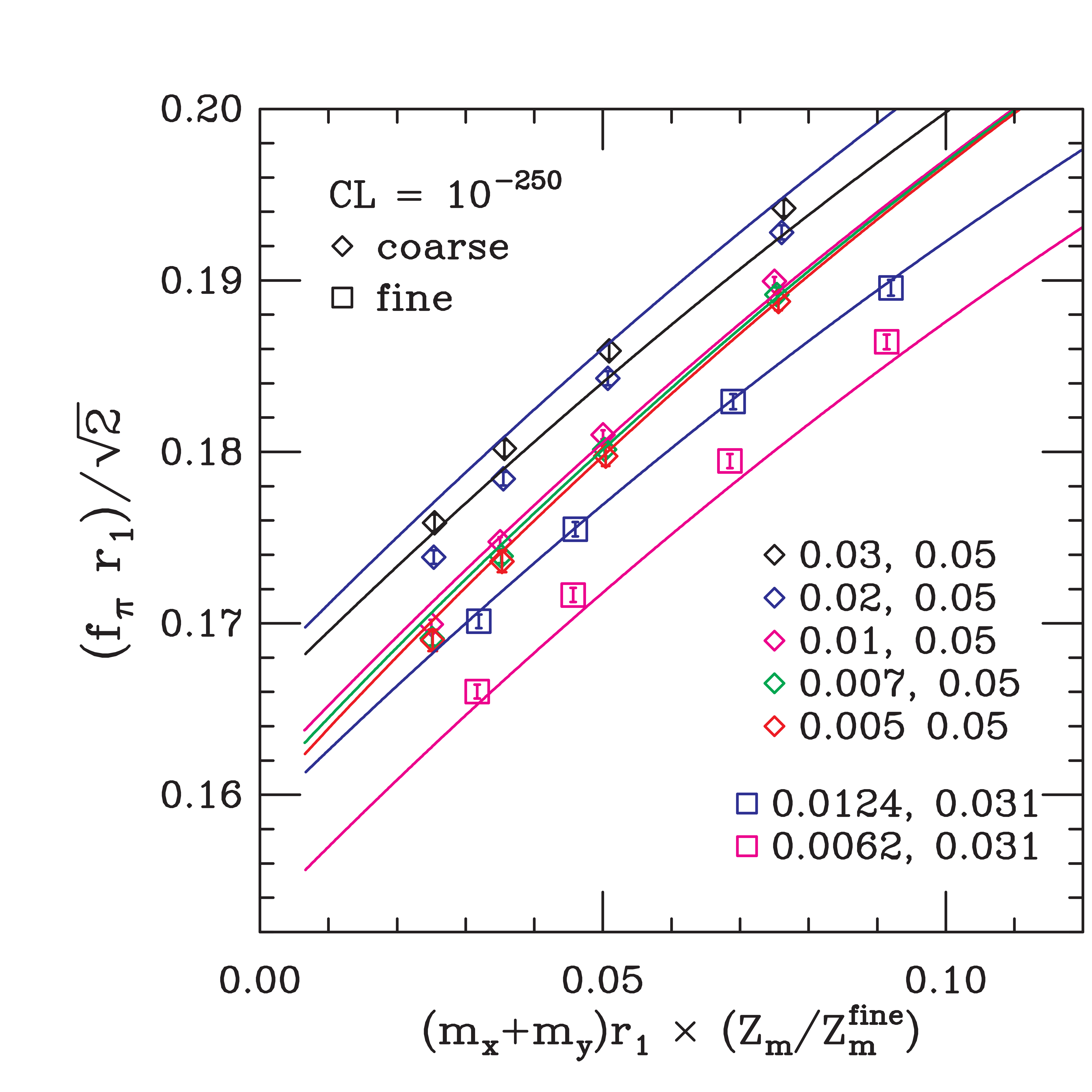
Figure 10: Fit of partially quenched data to continuum form. Data for both $f_{\pi}$ and $m_{\pi}^{2}/(m_{x}+m_{y})$ with various $m_{x}$ and $m_{y}$ values are included in the fit, but only $f_{\pi}$ points with $m_{x}=m_{y}$ are shown.

In physical units, the splittings on the coarse lattices are quite large. The largest is for the taste-singlet pion: $a^{2}\Delta_{I}\approx(450\;{\rm Me\!V})^{2}$; while the smallest, for the taste axial-vector pion, is $a^{2}\Delta_{A}\approx(280\;{\rm Me\!V})^{2}$. Given the size of these splittings, which are discretization errors, it is not surprising that the lattice data is not well fit by continuum chiral perturbation theory ($\chi$PT) forms. Figure 10 shows such an attempted fit for the Goldstone $f_{\pi}$ to the standard NLO partially quenched continuum form SHARPE_SHORESH plus analytic NNLO terms. More details about this fit will be explained below, when we discuss the corresponding fits that take into account taste violations. For the moment, we simply remark that the minuscule confidence level (${\rm CL}\approx 10^{-250}$; $\chi^{2}/{\rm d.o.f.}=8.77$ with 204 degrees of freedom) shows how hard it is to ignore lattice artifacts at the level of chiral logarithms.

VI Staggered chiral perturbation theory

Lee and Sharpe LEE_SHARPE found the chiral Lagrangian that describes a single staggered field. Their Lagrangian includes the effects of taste violations at ${\cal O}(a^{2})$ as well as the standard violations of chiral symmetry from mass terms at ${\cal O}(m_{q})$, where $m_{q}$ is a generic quark mass. They introduced a power counting that considers $m_{q}$ and $a^{2}$ to be of the same order, which is appropriate here: In Fig. 9 the splittings are comparable to the squared meson masses. Tree level (LO) is thus ${\cal O}(m_{q},a^{2})$; chiral logs appear at one-loop (NLO) and are ${\cal O}(m_{q}^{2},m_{q}a^{2},a^{4}).\;$

The Lee-Sharpe Lagrangian is not directly appropriate to the calculations here because it has only one flavor (one staggered field). Aubin and Bernard CB_FSB ; CA_CB1 ; CA_CB2 have generalized Ref. LEE_SHARPE to $n$ staggered flavors and shown how to accommodate the $\root 4 \of{\rm Det}$ trick in loop calculations. This is what is meant by “staggered chiral perturbation theory,” S$\chi$PT.

Continuum chiral perturbation theory can be thought of as an expansion in the dimensionless quantity

$$\chi_{q}\equiv\frac{2\mu m_{q}}{8\pi^{2}f_{\pi}^{2}}\ .$$ (11)

where ${2\mu m_{q}}$ is the tree-level mass of a $q\bar{q}$ meson. For physical kaons, we expect the relevant quark mass parameter to be $\chi_{ud,s}\equiv(\chi_{ud}+\chi_{s})/2\approx 0.18$ (where $\chi_{ud}$ is the average value for the $u$ and $d$ quarks); this is reasonable given the experimental result $f_{K}/f_{\pi}\approx 1.22$.

Staggered chiral perturbation theory is a joint expansion in $\chi_{q}$ and $\chi_{a^{2}}$, which measures the size of the ${\cal O}(a^{2})$ taste violations:

$$\chi_{a^{2}}\equiv\frac{a^{2}\overline{\Delta}}{8\pi^{2}f_{\pi}^{2}}\ ,$$ (12)

where $a^{2}\overline{\Delta}$ is a “typical” taste-violating term. Taking for $a^{2}\overline{\Delta}$ the average meson splitting (see Eq. (28) below), we have $a^{2}\overline{\Delta}\approx(350\;{\rm Me\!V})^{2}$ and $\chi_{a^{2}}\approx 0.09$ on the coarse lattices; $a^{2}\overline{\Delta}\approx(200\;{\rm Me\!V})^{2}$ and $\chi_{a^{2}}\approx 0.03$ on the fine lattices. If one instead uses the larger of the ${\cal O}(a^{2})$ taste-violating hairpin parameters CA_CB1 ; CA_CB2 , $a^{2}\delta^{\prime}_{A}$, to estimate $\overline{\Delta}$ and $\chi_{a^{2}}$, one gets slightly smaller values.

VI.1 NLO forms

One-loop chiral logs and analytic terms have been calculated in S$\chi$PT for Goldstone meson masses CA_CB1 and decay constants CA_CB2 . Partially quenched results are included, so all forms needed to fit the numerical data are available.

References CA_CB1 ; CA_CB2 express the chiral logarithms in terms of

$$\ell(m^{2}) \equiv m^{2}\left(\ln\frac{m^{2}}{\Lambda_{\chi}^{2}}+\delta_{1}(mL)\right)$$ (13)

$$\tilde{\ell}(m^{2}) \equiv -\left(\ln\frac{m^{2}}{\Lambda_{\chi}^{2}}+1\right)+\delta_{3}(mL)\ ,$$ (14)

where $\Lambda_{\chi}$ is the chiral scale, and $L$ is the spatial dimension. The finite volume correction terms $\delta_{1}$ and $\delta_{3}$ are CB_FSB

$$\delta_{1}(mL) = 4\sum_{\vec{r}\neq 0}\frac{K_{1}(|\vec{r}|mL)}{mL|\vec{r}|}\ ,$$ (15)

$$\delta_{3}(mL) = 2\sum_{\vec{r}\neq 0}K_{0}(|\vec{r}|mL)\ ,$$ (16)

where $K_{0}$ and $K_{1}$ are Bessel functions of imaginary argument, and $\vec{r}$, which labels the various periodic images, is a three-dimensional vector with integer components. We have assumed here that corrections due to the finite time extent are negligible; this is true for our lattices, for which the time dimension is between $2.7$ and $3.4$ times greater than the spatial dimension. The function $\ell(m^{2})$ in Eq. (13) arises from tadpole diagrams with a single meson propagator; $\tilde{\ell}(m^{2})$ in Eq. (14) comes from double-poles, which are present only in the partially quenched (and quenched) cases, not in the full QCD limit. In practice, we compute the sum in Eq. (15) or Eq. (16) with cutoff $|\vec{r}|\leq N$, where $N$ is an integer, and increment $N$ by 1 until the sum changes by a fractional amount $\leq\epsilon$. To be conservative, we take $\epsilon=10^{-9}$ for central-value fits. However, a much weaker criterion, $\epsilon=0.001$, is adequate to reduce the error in the sum well below our statistical errors, and we often use the weaker criterion for alternative fits in the systematic error estimates.

In the generic case relevant to our data ($m_{u}=m_{d}\equiv\hat{m}\not=m_{s}$ and no degeneracies between valence and sea quarks), the NLO S$\chi$PT expressions for a meson $P$ composed of valence quarks $x$ and $y$ are CA_CB1 ; CA_CB2

$$\frac{(m^{\rm NLO}_{P^{+}_{5}})^{2}}{\left(m_{x}+m_{y}\right)} = \mu\Biggl{\{}1+\frac{1}{16\pi^{2}f^{2}}\Bigg{(}\frac{2}{3}\sum_{j}R^{[3,2]}_{j}(\{{\cal M}^{[3]}_{XY_{I}}\})\;\ell(m^{2}_{j})$$ (17)

$$-2a^{2}\delta^{\prime}_{V}\sum_{j}R^{[4,2]}_{j}(\{{\cal M}^{[4]}_{XY_{V}}\})\,\ell(m^{2}_{j})-2a^{2}\delta^{\prime}_{A}\sum_{j}R^{[4,2]}_{j}(\{{\cal M}^{[4]}_{XY_{A}}\})\,\ell(m^{2}_{j})+a^{2}(L^{\prime\prime}+L^{\prime})\Bigg{)}$$

$$+\frac{16\mu_{\rm tree}}{f^{2}}\left(2L_{8}-L_{5}\right)\left(m_{x}+m_{y}\right)+\frac{32\mu_{\rm tree}}{f^{2}}\left(2L_{6}-L_{4}\right)\left(2\hat{m}+m_{s}\right)\Biggr{\}}$$

$$f^{\rm NLO}_{P^{+}_{5}} = f\Biggl{\{}1+\frac{1}{16\pi^{2}f^{2}}\Biggl{[}-\frac{1}{32}\sum_{Q,B}\ell\left(m^{2}_{Q_{B}}\right)+\frac{1}{6}\Biggl{(}R^{[2,2]}_{X_{I}}(\{{\cal M}^{[2]}_{X_{I}}\})\tilde{\ell}(m^{2}_{X_{I}})$$ (18)

$$+R^{[2,2]}_{Y_{I}}(\{{\cal M}^{[2]}_{Y_{I}}\})\tilde{\ell}(m^{2}_{Y_{I}})+\sum_{j}D^{[2,2]}_{j,X_{I}}(\{{\cal M}^{[2]}_{X_{I}}\})\ell(m^{2}_{j})$$

$$+\sum_{j}D^{[2,2]}_{j,Y_{I}}(\{{\cal M}^{[2]}_{Y_{I}}\})\ell(m^{2}_{j})-2\sum_{j}R^{[3,2]}_{j}(\{{\cal M}^{[3]}_{XY_{I}}\})\ell(m^{2}_{j})\Biggr{)}$$

$$+\frac{1}{2}a^{2}\delta^{\prime}_{V}\Biggl{(}R^{[3,2]}_{X_{V}}(\{{\cal M}^{[3]}_{X_{V}}\})\tilde{\ell}(m^{2}_{X_{V}})+R^{[3,2]}_{Y_{V}}(\{{\cal M}^{[3]}_{Y_{V}}\})\tilde{\ell}(m^{2}_{Y_{V}})$$

$$+\sum_{j}D^{[3,2]}_{j,X_{V}}(\{{\cal M}^{[3]}_{X_{V}}\})\ell(m^{2}_{j})+\sum_{j}D^{[3,2]}_{j,Y_{V}}(\{{\cal M}^{[3]}_{Y_{V}}\})\ell(m^{2}_{j})$$

$$+2\sum_{j}R^{[4,2]}_{j}(\{{\cal M}^{[4]}_{XY_{V}}\})\ell(m^{2}_{j})\Biggr{)}+\Bigl{(}V\to A\Bigr{)}+a^{2}(L^{\prime\prime}-L^{\prime})\Biggr{]}$$

$$+\frac{8\mu_{\rm tree}}{f^{2}}L_{5}\left(m_{x}+m_{y}\right)+\frac{16\mu_{\rm tree}}{f^{2}}L_{4}\left(2\hat{m}+m_{s}\right)\Biggr{\}}\ .$$

Here $\mu$ and $f$ are the continuum chiral parameters, $\delta^{\prime}_{V}$ and $\delta^{\prime}_{A}$ are LO taste-violating parameters (hairpins), $L_{i}$ are the NLO Gasser-Leutwyler GASSER_LEUTWYLER coefficients, and $L^{\prime}$ and $L^{\prime\prime}$ are linear combinations of the taste-violating NLO coefficients. The reason for using the tree-level $\mu_{\rm tree}$ parameter from Eq. (9) in the $L_{i}$ terms will be explained in Sec. VI.2. $X_{\Xi}$ and $Y_{\Xi}$ are flavor-neutral mesons of taste $\Xi$ made of $x,\bar{x}$ and $y,\bar{y}$ quarks, respectively, and $U_{\Xi}$, $D_{\Xi}$, and $S_{\Xi}$ are corresponding flavor-neutral mesons made from $u$, $d$, and $s$ sea quarks, respectively. The index $Q$ runs over the 6 mesons made from one valence and one sea quark, and $B$ runs over the 16 meson tastes. The residues $R^{[n,k]}_{j}$ and $D^{[n,k]}_{j,i}$ in Eqs. (17) and (18) are defined in Refs. CA_CB1 ; CA_CB2 . For completeness, we quote them here:

$$R_{j}^{[n,k]}\left(\left\{{\cal M}\right\}\!;\!\left\{\mu\right\}\right)\equiv\frac{\prod_{a=1}^{k}(\mu^{2}_{a}-m^{2}_{j})}{\prod_{\ell=1}^{{}^{\prime}n}(m^{2}_{\ell}-m^{2}_{j})}\ .$$ (19)

$$D_{j,i}^{[n,k]}\left(\left\{{\cal M}\right\}\!;\!\left\{\mu\right\}\right)\equiv-\frac{d}{dm^{2}_{i}}R_{j}^{[n,k]}\left(\left\{{\cal M}\right\}\!;\!\left\{\mu\right\}\right)\ .$$ (20)

Each of these residues is a function of two sets of masses, the “denominator” set $\{{\cal M}\}=\{m_{1},m_{2},\ldots,m_{n}\}$ and the “numerator” set $\{\mu\}=\{\mu_{1},\mu_{2},\ldots,\mu_{k}\}$. The indices $j$ and $i$, $1\leq j,i\leq n$, refer to particular denominator masses; the prime on the product in the denominator of Eq. (19) means that $\ell=j$ is omitted.

In Eqs. (17) and (18), the denominator mass-set arguments are shown explicitly; they are

$$\{{\cal M}^{[2]}_{X_{I}}\} \equiv \{m_{X_{I}},m_{\eta_{I}}\}\ ,$$

$$\{{\cal M}^{[2]}_{Y_{I}}\} \equiv \{m_{Y_{I}},m_{\eta_{I}}\}\ ,$$

$$\{{\cal M}^{[3]}_{XY_{I}}\} \equiv \{m_{X_{I}},m_{Y_{I}},m_{\eta_{I}}\}\ ,$$

$$\{{\cal M}^{[3]}_{X_{V}}\} \equiv \{m_{X_{V}},m_{\eta_{V}},m_{\eta^{\prime}_{V}}\}\ ,$$ (21)

$$\{{\cal M}^{[3]}_{Y_{V}}\} \equiv \{m_{Y_{V}},m_{\eta_{V}},m_{\eta^{\prime}_{V}}\}\ ,$$

$$\{{\cal M}^{[4]}_{XY_{V}}\} \equiv \{m_{X_{V}},m_{Y_{V}},m_{\eta_{V}},m_{\eta^{\prime}_{V}}\}\ .$$

The index $j$ in Eqs. (17) and (18) is summed over the denominator masses. Sets for axial-vector taste ($A$) are found from the corresponding vector taste ($V$) sets by taking $V\to A$ in Eq. (VI.1). The masses $m_{\eta_{I}}$, $m_{\eta_{V}}$, $m_{\eta^{\prime}_{V}}$ are given by CA_CB1

$$m_{\eta_{I}}^{2} = \frac{m_{U_{I}}^{2}}{3}+\frac{2m_{S_{I}}^{2}}{3}\ ,$$

$$m_{\eta_{V}}^{2} = \frac{1}{2}\left(m_{U_{V}}^{2}+m_{S_{V}}^{2}+\frac{3}{4}a^{2}\delta^{\prime}_{V}-Z\right)\ ,$$

$$m_{\eta^{\prime}_{V}}^{2} = \frac{1}{2}\left(m_{U_{V}}^{2}+m_{S_{V}}^{2}+\frac{3}{4}a^{2}\delta^{\prime}_{V}+Z\right)\ ;$$ (22)

$$Z \equiv \sqrt{\left(m_{S_{V}}^{2}-m_{U_{V}}^{2}\right)^{2}-\frac{a^{2}\delta^{\prime}_{V}}{2}\left(m_{S_{V}}^{2}-m_{U_{V}}^{2}\right)+\frac{9(a^{2}\delta^{\prime}_{V})^{2}}{16}}\ .$$

The numerator mass-set arguments of the residues in Eqs. (17) and (18) are not shown explicitly because they are always

$$\{\mu^{[2]}_{\Xi}\}\equiv\{m_{U_{\Xi}},m_{S_{\Xi}}\}\ ,$$ (23)

where the taste label $\Xi$ is taken equal to the taste of the denominator set.

Degeneracies among the various masses in Eqs. (17) and (18) occur quite often in our data set. In particular, “partially quenched pions” have $m_{x}=m_{y}$ and hence $m_{X_{B}}=m_{Y_{B}}$ for each taste $B$. Similarly “partially quenched kaons” have $m_{y}=m_{s}$ and hence $m_{Y_{B}}=m_{S_{B}}$. Going to full QCD introduces additional degeneracies $m_{X}=m_{Y}=m_{U}$ (for pions) or $m_{X}=m_{U}$ (for kaons). Further, the accidental degeneracy $m_{Y_{I}}=m_{\eta_{I}}$ appears in our data when $am_{y}=0.04$, $a\hat{m}^{\prime}=0.02$, $am^{\prime}_{s}=0.05$ (coarse) or $am_{y}=0.0248$, $a\hat{m}^{\prime}=0.0124$, $am^{\prime}_{s}=0.031$ (fine). Formulas for many of these degenerate cases appear in Refs. CA_CB1 ; CA_CB2 . For the other cases, one can carefully take appropriate limits in Eqs. (17) and (18), or, more conveniently, return to the original integrands in Refs. CA_CB1 ; CA_CB2 and take the limits before performing the momentum integrations.

Because Eqs. (17) and (18) are quite complicated, it is useful to write down a simple result that shows more clearly how taste violations change the continuum chiral behavior. The pion decay constant in full QCD with two (degenerate) flavors ($m_{x}=m_{y}=m_{u}=m_{d}\equiv\hat{m}$, with the strange quark integrated out) is particularly simple. In that case, the result corresponding to Eq. (18) is

$$f^{\rm 1-loop}_{\pi^{+}_{5}} =f\Biggl{\{}1+\frac{1}{16\pi^{2}f^{2}}\Biggl{[}-2\left(\frac{1}{16}\sum_{B}\ell(m^{2}_{\pi_{B}})\right)$$ (24)

$$\hskip 43.36243pt-4\Biggl{(}\ell(m^{2}_{\eta^{\prime}_{V}})-\ell(m^{2}_{\pi_{V}})\Biggr{)}-4\Biggl{(}\ell(m^{2}_{\eta^{\prime}_{A}})-\ell(m^{2}_{\pi_{A}})\Biggr{)}+a^{2}(L^{\prime\prime}-L^{\prime})\Biggr{]}$$

$$\hskip 43.36243pt+\frac{8\mu_{\rm tree}}{f^{2}}L_{5}(2\hat{m})+\frac{16\mu}{f^{2}}L_{4}\left(2\hat{m}\right)\Biggr{\}}\ ,$$

with $B$ running as usual over the 16 possible tastes, and

$$m_{\pi_{B}}^{2} \equiv m_{U_{B}}^{2}=m_{D_{B}}^{2}\ ,$$

$$m_{\eta^{\prime}_{V}}^{2} = m_{\pi_{V}}^{2}+\frac{1}{2}a^{2}\delta^{\prime}_{V}\ ,$$

$$m_{\eta^{\prime}_{A}}^{2} = m_{\pi_{A}}^{2}+\frac{1}{2}a^{2}\delta^{\prime}_{A}\ .$$ (25)

In Eq. (24), the term multiplied by $-2$ gives the average of all tastes and becomes the standard $SU(2)_{L}\times SU(2)_{R}$ chiral logarithm in the continuum limit, when all tastes are degenerate. The terms multiplied by $-4$ clearly vanish in the continuum limit because $m_{\pi_{V}}=m_{\eta^{\prime}_{V}}$ and $m_{\pi_{A}}=m_{\eta^{\prime}_{A}}$ when $a^{2}\delta^{\prime}_{V}=0=a^{2}\delta^{\prime}_{A}$.

Since $\hat{m}^{\prime}$ is significantly less than $m^{\prime}_{s}$ for many of our runs, Eq. (24) is often not a bad approximation to the chiral behavior of our (full QCD) data. It will be useful in the discussion of finite volume effects in Sec. IX.4.6.

We note here that Refs. LEE_SHARPE ; CA_CB1 ; CA_CB2 explicitly include in the chiral Lagrangian the effects of terms in the ${\cal O}(a^{2})$ staggered-quark Symanzik action that violate the taste symmetries. There are also “generic” ${\cal O}(a^{2})$ terms in the Symanzik action that have the same symmetries as the continuum QCD action and are not included explicitly. An example is $a^{2}\bar{\psi}D^{2}D_{\mu}(\gamma_{\mu}\otimes I)\psi$, where $\gamma_{\mu}$ and $I$ act on spin and taste indices, respectively. The effect of such terms on the chiral Lagrangian is to produce ${\cal O}(a^{2})$ variation in physical parameters such as $f$, $\mu$, and, at higher order in $m_{q}$, $L_{i}$. We build the possibility of such generic variation in physical parameters into the chiral fits below. Since our staggered action is $a^{2}$ tadpole improved, we expect such generic variation to be of size $\alpha_{S}a^{2}\Lambda_{\rm QCD}\approx 2\%$. When we extrapolate the physical parameters to the continuum, we will need to know how $\alpha_{S}a^{2}$ changes from the coarse to fine lattice. As in the case of taste violations, such discretization errors occur at the scale of the cutoff. Therefore, we use $\alpha_{S}=\alpha_{V}(q^{*}=\pi/a)$ for central values, and allow $q^{*}$ to vary between $\pi/(2a)$ and $2\pi/a$ for the error estimate. We have

$$\frac{(\alpha_{V}(q^{*}\!\!=\!\pi/a)\;a^{2})_{\rm fine}}{(\alpha_{V}(q^{*}\!\!=\!\pi/a)\;a^{2})_{\rm coarse}}=0.427\ ,$$ (26)

and a range for this ratio of 0.398 to 0.441.

As they stand, Eqs. (17) and (18) are slightly inconvenient because the renormalization of the ${\cal O}(m_{q}a^{2})$ analytic NLO parameters $L^{\prime}$ and $L^{\prime\prime}$ under a change in the chiral scale $\Lambda_{\chi}$ is complicated and involves the physical $L_{i}$ parameters. This is due to the fact that the meson masses multiplying the logarithms include ${\cal O}(a^{2})$ splittings. It is more natural, therefore, to redefine the $L^{\prime}$ and $L^{\prime\prime}$ by associating particular ${\cal O}(a^{2})$ terms with the $L_{i}$. We make the replacements

$$\frac{16\mu_{\rm tree}}{f^{2}}(2L_{8}-L_{5})(m_{x}+m_{y}) \to \frac{16}{f^{2}}(2L_{8}-L_{5})\Big{[}\mu_{\rm tree}(m_{x}+m_{y})+a^{2}\Delta_{I}\Big{]}\ ,$$

$$\frac{32\mu_{\rm tree}}{f^{2}}\left(2L_{6}-L_{4}\right)\left(2\hat{m}+m_{s}\right) \to \frac{32}{f^{2}}(2L_{6}-L_{4})\Big{[}\mu_{\rm tree}(2\hat{m}+m_{s})+{\scriptstyle\raise 0.45206pt\hbox{${3\over 2}$}}a^{2}\Delta_{I}\Big{]}\ ,$$

$$\frac{8\mu_{\rm tree}}{f^{2}}L_{5}\left(m_{x}+m_{y}\right) \to \frac{8}{f^{2}}L_{5}\Big{[}\mu_{\rm tree}(m_{x}+m_{y})+a^{2}\Delta_{av}\Big{]}\ ,$$

$$\frac{16\mu_{\rm tree}}{f^{2}}L_{4}\left(2\hat{m}+m_{s}\right) \to \frac{16}{f^{2}}L_{4}\Big{[}\mu_{\rm tree}(2\hat{m}+m_{s})+{\scriptstyle\raise 0.45206pt\hbox{${3\over 2}$}}a^{2}\Delta_{av}\Big{]}\ ,$$ (27)

where $a^{2}\Delta_{I}$ is given by Eq. (9), and

$$a^{2}\Delta_{av}\equiv\frac{a^{2}}{16}(\Delta_{5}+4\Delta_{A}+6\Delta_{T}+4\Delta_{V}+\Delta_{I})$$ (28)

is the average splitting. After these redefinitions, a change in $\Lambda_{\chi}$ renormalizes $L^{\prime}$ according to:

$$L^{\prime}(\tilde{\Lambda}_{\chi})=L^{\prime}(\Lambda_{\chi})+2(\delta^{\prime}_{A}+\delta^{\prime}_{V})\;\ln(\tilde{\Lambda}_{\chi}^{2}/\Lambda_{\chi}^{2})\ ;$$ (29)

while $L^{\prime\prime}$ is independent of scale. From this we would expect that $L^{\prime}$ is comparable in size to $\delta^{\prime}_{A}+\delta^{\prime}_{V}$, an expectation that is borne out by the fits. The $L_{i}$ renormalize by:

$$L_{i}(\tilde{\Lambda}_{\chi})=L_{i}(\Lambda_{\chi})+\frac{C_{i}}{256\pi^{2}}\ln(\tilde{\Lambda}_{\chi}^{2}/\Lambda_{\chi}^{2})\ ,$$ (30)

with

$$C_{4}=-1\;; C_{5}=-3\;;$$ (31)

$$2C_{6}-C_{4}=-2/9\;; 2C_{8}-C_{5}=4/3\;.$$ (32)

VI.2 NNLO Terms

As we will see below, the high statistical precision of our data requires us to go beyond the NLO formulas, even for subsets of the data that include only the lighter valence quark masses. We include explicitly all NNLO physical analytic parameters, i.e., all analytic terms of ${\cal O}(m_{q}^{3})$. There are five such terms for $m^{2}_{P^{+}}$ and an additional five for $f_{P^{+}}$ Aubin:2003ne . Expressed in terms of $\chi_{q}$ defined in Eq. (11), they are given by:

$$\frac{(m^{\rm NNLO}_{P^{+}_{5}})^{2}}{\left(m_{x}+m_{y}\right)} = \mu\Big{(}1+{\rm NLO}+\beta^{(m)}_{1}\left(\chi_{x}+\chi_{y}\right)^{2}+\beta^{(m)}_{2}\left(2\chi_{ud}+\chi_{s}\right)^{2}+\beta^{(m)}_{3}\left(\chi_{x}+\chi_{y}\right)\left(2\chi_{ud}+\chi_{s}\right)$$ (33)

$$\qquad\quad+\;\beta^{(m)}_{4}\left(\chi_{x}-\chi_{y}\right)^{2}+\beta^{(m)}_{5}\left(2\chi^{2}_{ud}+\chi^{2}_{s}\right)\Big{)}\ ,$$

$$f^{\rm NNLO}_{P^{+}_{5}} = f\Big{(}1+{\rm NLO}+\beta^{(f)}_{1}\left(\chi_{x}+\chi_{y}\right)^{2}+\beta^{(f)}_{2}\left(2\chi_{ud}+\chi_{s}\right)^{2}+\beta^{(f)}_{3}\left(\chi_{x}+\chi_{y}\right)\left(2\chi_{ud}+\chi_{s}\right)$$ (34)

$$\qquad\quad+\;\beta^{(f)}_{4}\left(\chi_{x}-\chi_{y}\right)^{2}+\beta^{(f)}_{5}\left(2\chi^{2}_{ud}+\chi^{2}_{s}\right)\Big{)}\ ,$$

where “NLO” denotes the lower order contributions, (the corrections to the leading “1” in Eqs. (17) and (18), with the substitutions in Eq. (27)). The interchange symmetries among valence quarks $x\leftrightarrow y$ and sea quarks $u\leftrightarrow d\leftrightarrow s\leftrightarrow u$ restrict the form of the NNLO corrections. These terms were obtained independently in Ref. Sharpe:2003vy .

Possible analytic taste-violating terms at NNLO of ${\cal O}(m_{q}^{2}a^{2})$ are included implicitly by allowing the $L_{i}$ (${\cal O}(m_{q}^{2})$ terms) to vary with lattice spacing. However, such variation can be caused either by taste-violating terms in the Symanzik Lagrangian or by terms with the same symmetries as the continuum operators but with explicit factors of $a^{2}$ (i.e., by generic discretization errors on the $L_{i}$). As explained above, the generic discretization errors are expected to be $\approx\!2\%$; while the new taste-violating terms could change the apparent value of $L_{i}$ between coarse and fine sets by order $\chi^{\rm coarse}_{a^{2}}-\chi^{\rm fine}_{a^{2}}\approx 6\%$. For our preferred fits, we use Bayesian priors BAYSE to restrict the differences in the $L_{i}$ on coarse and fine sets to be at most $7.5\%$ (for a 3-$\sigma$ variation); while in alternative fits used to assess the systematic error, we relax or tighten this restriction. (See Sec. IX.2.) Note that when we extrapolate the $L_{i}$ to the continuum, we have no a priori way to distinguish variation as $\alpha_{S}a^{2}$ (generic discretization errors) from variation as $\alpha_{S}^{2}a^{2}$ (taste violations). Therefore, we consider both types of variation (i.e., Eqs. (26) and (10), as well as the ranges of these ratios) and include the difference in the systematic error. In practice, these alternative fits and these assumptions in how the $L_{i}$ are extrapolated to the continuum contribute only a small fraction of the total systematic error. (See Table 7.)

At NNLO, ${\cal O}(m_{q}a^{4})$ analytic terms may also affect $m^{2}_{P^{+}_{5}}$ and $f_{P^{+}_{5}}$. We neglect such terms, which would make contributions similar to that of $L^{\prime}$ and $L^{\prime\prime}$ in Eqs. (17) and (18), but multiplied by $a^{4}$ instead of $a^{2}$. Because $\chi_{a^{2}}$ is only 0.09 in the worst case, we would expect the error thereby induced to be at most $\chi^{2}_{a^{2}}\sim 1\%$. In fact, since we consider a generous range for how taste-violating $a^{2}$ terms may vary as we go from coarse to fine lattices (see discussion immediately following Eq. (10)), the effects of ${\cal O}(m_{q}a^{4})$ analytic terms should already be included in our systematic error estimates.

The final possible NNLO terms in the Lagrangian are ${\cal O}(a^{6})$. However, it is easy to see that such terms do not contribute to $m^{2}_{P^{+}_{5}}$ and $f_{P^{+}_{5}}$. The Goldstone theorem requires that $m^{2}_{P^{+}_{5}}$ be proportional to at least a single power of quark mass ($m_{x}+m_{y}$ in this case), and terms in the Lagrangian must have at least two derivatives to make analytic contributions to $f_{P^{+}_{5}}$ through Noether’s theorem or wave-function renormalization.

In addition to analytic terms at NNLO, there are, of course, NNLO chiral logarithms (from 2-loop graphs, as well as 1-loop graphs that involve NLO parameters). These non-analytic terms have not been calculated in S$\chi$PT, but in any case are not expected to be important here: Wherever the quark masses or splittings are large enough for the analytic NNLO terms to be significant, the NNLO logarithms should be slowly varying and well approximated by analytic terms. As discussed in Sec. IX.2, the NNLO terms make a difference primarily in the interpolation around $m_{s}$, not in the extrapolation to $\hat{m}$. The systematic errors inherent in our treatment of the NNLO terms are estimated by varying the masses we fit to and the Bayesian priors governing these terms and their changes with $a$, as well as by adding still higher (NNNLO) terms.

There are also NNLO effects induced by the ambiguity in the parameters one puts into NLO expressions. In particular, we have at present expressed the “chiral coupling,” $1/(16\pi^{2}f^{2})$ in Eqs. (17) and (18), in terms of bare (tree-level) parameter $f$. Replacing $f$ with the experimental value of $f_{\pi}$, say, would generate a difference at NNLO. As we discuss below, the difference between $f_{\pi}$ and $f$ is significant: $\approx\!13\%$. If we had the full NNLO expression, including 2-loop effects, then the ambiguity would be resolved up to terms of NNNLO. But in the present case there is no a priori way to decide this issue.

We argue, however, that putting a physical parameter in the chiral coupling ($f\to f_{\pi}$) is likely to result in a better convergent $\chi$PT. This is similar to the argument for using a physical, rather than bare, coupling in weak-coupling perturbation theory LEPAGE_MACKENZIE . In practice, we consider three versions of the fits:

• (1) Fix coupling as $1/(16\pi^{2}f_{\pi}^{2})$.

• (2) Leave coupling as $1/(16\pi^{2}f^{2})$.

• (3) Write coupling as $\omega/(16\pi^{2}f_{\pi}^{2})$ and treat $\omega$ as an additional fit parameter: either allow it to vary freely or force it to vary around 1 using Bayesian priors.

Good fits are possible with all three choices. Both because of the argument above, and because it guarantees that the NLO chiral logarithms for very light quarks have the expected weight relative to the tree level terms, we take choice (1) for our central values. Choice (3), with its extra parameter, results in the highest confidence levels of the three. When $\omega$ is allowed to vary freely, its value decreases as higher quark masses are included in the fits, reaching $\omega\approx 0.6$ by set II (see Sec. IX.1). This is similar to replacing $f\to f_{K}$, perhaps not surprising for fits that must cover a range of valence masses up to a large fraction of $m_{s}$. But for the quantities computed here, all of which are sensitive to the chiral behavior at low quark mass, we do not include fits with $\omega$ free since we expect $1/(16\pi^{2}f_{\pi}^{2})$, not $1/(16\pi^{2}f_{K}^{2})$, to be the correct weight for the logarithms in the low mass regime. We still allow fits with range $\omega=1.0\pm 0.1$ because 10% is roughly the difference between the physical $f^{2}_{\pi}$ and its value in the chiral limit. As discussed in Sec. X, the main effects of including fits with arbitrary $\omega$ would be to increase the systematic error in $f_{\pi}$ by about $1\;{\rm Me\!V}$ (with a corresponding effect on $f_{K}/f_{\pi}$) and to double the simulation error on $m_{u}/m_{d}$ (which error, however, is small compared to unknown electromagnetic effects).

Good fits with choice (2) require $f\,\raise 1.29167pt\hbox{$>$\kern-7.5pt\lower 4.30554pt\hbox{$\sim$}}\,f_{K}$ (equivalent to $\omega\approx 0.6$ in choice (3)) and quite large NNLO terms. In addition, the ${\cal O}(a^{2})$ NLO parameter $a^{2}L^{\prime\prime}$ becomes unreasonably large ($\sim(630\,{\rm Me\!V})^{2}$ on the coarse lattices). For these reasons we exclude choice (2) fits from the systematic error estimates; including them would increase systematic errors by amounts comparable to those of arbitrary $\omega$ fits.

Similar considerations apply to the parameter $\mu$. In the analytic terms involving the $L_{i}$ in Eqs. (17) and (18) (and hence in Eqs. (33) and (34)), we argue that it is best to put in $\mu_{\rm tree}$ from the linear (tree-level) fits, Eq. (9). The $L_{i}$ are then multiplied by actual squared meson masses (within the errors of Eq. (9)). This corresponds to how such terms are interpreted in continuum $\chi$PT analysis (see, e.g., Ref. GASSER_LEUTWYLER ). An alternative, a posteriori, choice would be to use the chiral limit of $m^{2}_{\pi}/(2\hat{m})$ coming from the full NNLO fit. This would replace $\mu_{\rm tree}$ in Eqs. (17) and (18) by a number 5% smaller. Since Eq. (9) gives a maximum of 7% errors, we choose that larger value as the systematic effect. It would however be unreasonable to replace $\mu_{\rm tree}$ in Eqs. (17) and (18) or (Eqs. (33) and (34)) by the fit parameter $\mu$ itself. That is because the effective value of $\mu$ is corrected by terms involving $m_{s}$ that do not go away in the chiral limit for the light quarks. Indeed, one might expect corrections of at least $\chi_{ud,s}+\chi^{2}_{ud,s}\approx 20\%$. In practice the fit parameter $\mu$ from our preferred NNLO fit on the intermediate valence mass set (subset II, Sec. IX.1) is 29% less than $\mu_{tree}$, which means that $\mu(m_{x}+m_{y})$ is significantly less than our measured value of $m^{2}_{P^{+}_{5}}\cong\mu_{\rm tree}(m_{x}+m_{y})$. This difference improves to 13% in the fit to the lightest masses.

As discussed in the introduction, all meson masses appearing in the NLO chiral logarithms in Eqs. (17) and (18) are similarly evaluated using the previously determined values of the taste splittings, $a^{2}\Delta_{B}$, and $\mu_{\rm tree}$ from the fit of our “full QCD” data for all meson tastes to Eq. (9). In our results for masses and decay constants, the NNLO error introduced by this procedure is negligible. That is because the effect of the small errors in masses in the chiral logarithms on our extrapolated values is almost completely canceled by the effect of variations of the analytic parameters in the fit. We can check this by replacing $\mu_{\rm tree}$ in the fit by the ($5\%$ different) chiral limit value; the effect is about $0.2\%$ on quark masses and less than $0.1\%$ on the decay constants, in both cases much less than the total systematic error. For the $L_{i}$, changing the value of $\mu$ in the chiral logarithms does not completely cancel the effect of changing its value in the analytic terms, but there is some cancellation. Therefore the $7\%$ systematic effect in the $L_{i}$ discussed in the previous paragraph remains a conservative estimate of the error.

VI.3 NNNLO terms

We sometimes add some NNNLO terms of the following form:

$$\frac{(m^{\rm NNNLO}_{P^{+}_{5}})^{2}}{\left(m_{x}+m_{y}\right)} = \mu\Big{(}1+{\rm NLO}+{\rm NNLO}+\rho^{(m)}\left(\chi_{x}+\chi_{y}\right)^{3}\Big{)}\ ,$$ (35)

$$f^{\rm NNLO}_{P^{+}_{5}} = f\Big{(}1+{\rm NLO}+{\rm NNLO}+\rho^{(f)}\left(\chi_{x}+\chi_{y}\right)^{3}\Big{)}\ ,$$ (36)

where NLO and NNLO represent the contributions from Eqs. (17), (18), (33) and (34). Since there are, of course, many additional NNNLO terms, it is nonsystematic to include only one each for $m_{P^{+}_{5}}$ and $f_{P^{+}_{5}}$. However, we pick these terms involving valence masses because there is a steeper dependence on the valence masses than on the sea quark masses. For lower quark masses, where we expect $\chi$PT to work well, we fit to Eqs. (35) and (36) only to estimate systematic errors due to the truncation of $\chi$PT. When the fits include valence masses equal to or greater than $m^{\prime}_{s}$, we also use Eqs. (35) and (36) in order to improve the interpolation around the strange quark mass. In the former case, we find that the values of $|\rho^{(f)}|$ and $|\rho^{(m)}|$ coming from the fits are typically less than 0.1; in both cases they are always less than 0.2 (including when we fit to Eqs. (37) and (38) — see Table 4).

Another form, used only for interpolations around the strange quark mass, adds on the square of the NLO term as a mock-up of the effect of 2-loop chiral logarithms:

$$\frac{(m^{\rm NNNLO^{\prime}}_{P^{+}_{5}})^{2}}{\left(m_{x}+m_{y}\right)} = \mu\Big{(}1+{\rm NLO}+{\rm NNLO}+\sigma^{(m)}\left({\rm NLO}\right)^{2}+\rho^{(m)}\left(\chi_{x}+\chi_{y}\right)^{3}\Big{)}\ ,$$ (37)

$$f^{\rm NNNLO^{\prime}}_{P^{+}_{5}} = f\Big{(}1+{\rm NLO}+{\rm NNLO}+\sigma^{(f)}\left({\rm NLO}\right)^{2}+\rho^{(f)}\left(\chi_{x}+\chi_{y}\right)^{3}\Big{)}\ ,$$ (38)

where again NLO and NNLO represent the contributions from Eqs. (17), (18), (33) and (34). The absolute values of the new coefficients $\sigma^{(m)}$ and $\sigma^{(f)}$ in the fits are never greater than 0.14.

VII Perturbation theory

Because the axial current we use to compute decay constants is partially conserved, there is no need for current renormalization. Mass renormalization is however needed to find continuum ($\overline{\text{MS}}$) quark masses, as discussed in Ref. strange-mass . Let $Z_{m}$ be the mass renormalization factor that connects the bare lattice mass $(am)_{0}$ and the $\overline{\text{MS}}$ mass at scale $\Lambda$:

$$m^{\text{$\overline{\text{MS}}$}}(\Lambda)=Z_{m}({a\Lambda})\frac{(am)_{0}}{au_{0P}}\ .$$ (39)

Here, unlike in Ref. strange-mass , we have shown explicitly the plaquette tadpole improvement factor $u_{0P}$, necessary because the MILC improved staggered action defines the lattice quark mass in a somewhat unconventional manner.

The renormalization factor $Z_{m}$ enters the analysis in another way. As mentioned above, we need to renormalize the parameter $\mu$ if we wish to compare its values at different lattice spacings. More precisely, we need the ratio

$$R_{m}\equiv\frac{Z_{m}(a^{\rm coarse}\Lambda)}{Z_{m}(a^{\rm fine}\Lambda)}\;\frac{u_{0P}^{\rm fine}}{u_{0P}^{\rm coarse}}\ ,$$ (40)

$R_{m}$ is in principle independent of $\Lambda$, although when $Z_{m}$ is evaluated at any given order in perturbation theory, there is residual $\Lambda$ dependence from neglected higher order terms. For definiteness, we take $\Lambda=2\,{\rm Ge\!V}$. $Z_{m}$ is given by strange-mass

$$Z_{m}(a\Lambda)=\left(1+\alpha_{V}(q^{*})\,Z_{m}^{(2)}(a\Lambda)+{\cal O}(\alpha^{2})\right)\ ,$$ (41)

where $\alpha_{V}$ is determined from small Wilson loops using third order perturbation theory Davies:2002mv ; new_alpha , the optimal scale $q^{*}$ is estimated using a second order BLM method Hornbostel:2002af , and $Z_{m}^{(2)}$ is Hein:2001kw ; Becher:2002if ; Q:thesis

$$Z_{m}^{(2)}(a\Lambda)=\left(b-\frac{4}{3\pi}-\frac{2}{\pi}\ln(a\Lambda)\right),$$ (42)

with $b\approx 0.5432$, correct to 0.1%. We have neglected the (tiny) ${\cal O}(a)$ mass dependence of $b$, and hence of $Z_{m}(a{\Lambda})$. From Ref. strange-mass , $q^{*}=2.335/a$ and $\alpha_{V}(q^{*})=0.252(5)$ on the coarse lattices; $q^{*}=1.80/a$ and $\alpha_{V}(q^{*})=0.247(4)$ on the fine.

To evaluate $R_{m}$, we use scale and plaquette values from the coarse $0.01/0.05$ and the fine $0.0062/0.031$ lattices, and neglect the the small variation among the coarse or fine sets. As mentioned previously, the $\Upsilon$ splittings give BIG_PRL ; HPQCD_PRIVATE $(a^{\rm coarse})^{-1}=1.588\,{\rm Ge\!V}$ and $(a^{\rm fine})^{-1}=2.271\,{\rm Ge\!V}$. The tadpole improvement factor are $u_{0P}^{\rm coarse}=0.8677$ and $u_{0P}^{\rm fine}=0.8782$. From Eqs. (40), (41) and (42), we find $R_{m}\approx 0.958$. Then,

$$\mu^{\rm coarse}=R_{m}\mu^{\rm fine}$$ (43)

with the above value of $R_{m}$ defines what we mean by “equality” of the parameter $\mu$ on coarse and fine lattices. Of course, Eq. (43) may be violated by generic ${\cal O}(a^{2})$ scaling violations ($\sim\!2\%$), as well as by perturbative errors. A priori, one expects a two-loop correction to $R_{m}$ of order $\alpha_{V}^{2}$. This is $\approx\!6\%$. In practice, fits have a confidence level that is higher than those of our preferred fits if we take $R_{m}\approx 0.87$ to $0.89$, i.e., a 7 to 9% difference from $R_{m}=0.958$. Although it is not possible to separate the perturbative errors from the discretization errors in this difference, here and in Ref. strange-mass we take the larger value, $9\%$, as the conservative estimate of perturbative errors. This is $\approx\!1.5\alpha_{V}^{2}$. For quantities that do not directly involve perturbation theory, such as the decay constants and the ratio $m_{u}/m_{d}$, we do not quote perturbative errors, per se. But $R_{m}$ still enters the chiral fits, so we include fits with $R_{m}=0.87$ among the alternatives.

Another rough estimate of $R_{m}$ comes from $\mu_{\rm tree}$, Eq. (9). Without the proliferation of parameters at NLO and NNLO, the tree-level form makes possible well-controlled fits on coarse and fine lattices separately. We get $R_{m}\approx 0.977$. But note that Eq. (9) can have up to $\sim\!7\%$ errors in describing the data, and there are also discretization errors in this estimate.

VIII Electromagnetic and isospin-violating effects

Given the precision we are aiming at here, it is necessary to take into account electromagnetic (EM) and isospin-violating effects, at least in an approximate way. Our simulation is in isospin-symmetric QCD, with $m_{u}$ set equal to $m_{d}$, and the electromagnetic coupling, $e^{2}=4\pi\alpha_{EM}$, set to 0. This means that when we compare meson masses to experiment to determine the physical quark masses $\hat{m}$ and $m_{s}$, we must first adjust the experimental numbers to what they would be in a world without EM effects or isospin violation. This is particularly important for the pion, since the difference between $m_{\pi^{+}}^{2}$ and $m_{\pi^{0}}^{2}$ is almost 7%. Because the adjustment is only approximate, there are some residual systematic errors on the quark masses, as discussed in Ref. strange-mass .

The decay constants, as well as the low energy constants $L_{i}$, are by definition pure QCD quantities, so we do not have to take EM effects directly into account in our determination. Nevertheless, there are indirect EM effects on $f_{\pi}$ and $f_{K}$, which come in through the quark masses when we extrapolate to the physical point. Isospin violations are irrelevant for the $L_{i}$, which are defined to be mass independent. But for the decay constants, there are both direct and indirect isospin-violating effects, which we estimate below. The end result is that both the (indirect) EM and isospin-violating errors on decay constants are very small, as long as we are careful to extrapolate to the appropriate values of the quark mass in each case. However the EM error on $m_{u}/m_{d}$ is large unless we are willing to assume that the EM effects on meson masses are accurately known.

Electromagnetism can be included in $\chi$PT in a systematic way. Dashen’s theorem Dashen:eg summarizes the EM effects on meson masses at lowest nontrivial order in $e^{2}$ and the quark masses. It states that $m^{2}_{\pi^{+}}$ and $m^{2}_{K^{+}}$ receive equal ${\cal O}(e^{2})$ contributions in the chiral limit; while the $\pi^{0}$ and $K^{0}$ masses are unaffected. However, there can be large and different EM contributions to $m^{2}_{\pi^{+}}$ and $m^{2}_{K^{+}}$ of order $e^{2}\chi_{ud,s}$ Donoghue:hj ; Urech:1994hd ; Bijnens:1996kk ; Gao:1996sa . Following Ref. Nelson-thesis , we let $\Delta_{E}$ parameterize violations of Dashen’s theorem:

$$(m^{2}_{K^{+}}-m^{2}_{K^{0}})_{\rm EM}=(1+\Delta_{E})(m^{2}_{\pi^{+}}-m^{2}_{\pi^{0}})_{\rm EM}\ .$$ (44)

Then Refs. Donoghue:hj ; Urech:1994hd ; Bijnens:1996kk ; Gao:1996sa suggest $\Delta_{E}\approx 1$. Most of these corrections are probably to the charged meson masses. Indeed, the violation of Dashen’s theorem for the $\pi^{0}$ is ${\cal O}(e^{2}\chi_{ud})$ Urech:1994hd and therefore small. The EM contribution to $m^{2}_{K^{0}}$, on the other hand, is in principle the same order as the violations of Dashen’s theorem for the charged masses, $e^{2}\chi_{ud,s}$ Urech:1994hd . Nevertheless, a large $N_{c}$, extended NJL model calculation Bijnens:1996kk finds a tiny EM correction to the $K^{0}$ mass at this order. To be conservative, though, we allow for EM contributions to $m^{2}_{K^{0}}$ of order of half the violations of Dashen’s theorem, with unknown sign:

$$(m_{K^{0}}^{2})_{\rm EM}\sim\pm(\Delta_{E}/2)(m^{2}_{\pi^{+}}-m^{2}_{\pi^{0}})_{\rm EM}\ .$$ (45)

The effects of isospin violation in the pion masses are quite small. When $m_{u}\not=m_{d}$, $m^{2}_{\pi^{0}}$ gets a contribution of order $(\chi_{u}-\chi_{d})^{2}$. The isospin-violating splitting $(m_{\pi^{+}}-m_{\pi^{0}})_{\rm QCD}$ is estimated as $0.17(3)\,{\rm Me\!V}$ in Ref. GASSER_LEUTWYLER , and as $0.32(20)\,{\rm Me\!V}$ in Ref. Amoros:2001cp . In the kaon system, on the other hand, the effects of isospin violation are clearly important, as is obvious from the fact that the experimental $K^{+}$–$K^{0}$ splitting is of opposite sign to that in Eq. (44) for any $\Delta_{E}>-1$. In our calculation, we can reduce the isospin violating effects in the kaon masses to the same order as in the pion system by focusing on the isospin averaged quantity $(m_{K^{0}}^{2}+m_{K^{+}}^{2})/2$. We then neglect the remaining isospin violations in the meson masses. We have checked, using the estimates for $(m_{\pi^{+}}-m_{\pi^{0}})_{\rm QCD}$ above, that the indirect effect of such isospin violations on decay constants is extremely small: $\raise 1.29167pt\hbox{$<$\kern-7.5pt\lower 4.30554pt\hbox{$\sim$}}0.03\%$. These isospin violations were also neglected in the computation of quark masses in Ref. strange-mass . We note, however, that including isospin violations could have some small effect there, in particular on the result for the ratio $m_{s}/\hat{m}$. If $(m_{\pi^{+}}-m_{\pi^{0}})_{\rm QCD}$ is at the upper end of the range in Amoros:2001cp , the central value for $m_{s}/\hat{m}$ in Ref. strange-mass could be changed from 27.4 to as low as 27.2.

Based on the above discussion, we may determine the physical values of $\hat{m}$ and $m_{s}$ by extrapolating the lattice squared meson masses to $m^{2}_{\hat{\pi}}$ and $m^{2}_{\hat{K}}$, given by

$$m^{2}_{\hat{\pi}} \equiv m^{2}_{\pi^{0}}$$

$$m^{2}_{\hat{K}} \equiv {\scriptstyle\raise 0.60275pt\hbox{${1\over 2}$}}\left(m_{K^{0}}^{2}+m_{K^{+}}^{2}-(1+\Delta_{E})(m_{\pi^{+}}^{2}-m_{\pi^{0}}^{2})\right)\ ,$$ (46)

where experimental values are to be used on the right hand side. Allowing for EM corrections to the $K^{0}$ mass, Eq. (45), replaces $\Delta_{E}\approx 1$ in Eq. (VIII) with an effective value in the range 0–2, which is in any case a conservative range for $\Delta_{E}$ that includes the Dashen theorem result. Here and in Ref. strange-mass , we take $\Delta_{E}=1$ for the central value, and use $0\leq\Delta_{E}\leq 2$ to estimate systematic errors in $\hat{m}$, $m_{s}$, and their ratio.

We can also estimate $m_{u}$ (or equivalently the ratios $m_{u}/m_{d}$ or $m_{u}/\hat{m}$) from our simulation. Given $m_{s}$, we find $m_{u}$ by extrapolating in the light valence mass to the point where the $K^{+}$ has the mass $(m_{K^{+}})_{\rm QCD}$, where “QCD” indicates that EM effects have been removed. We take

$$(m^{2}_{K^{+}})_{\rm QCD}\equiv m_{K^{+}}^{2}-(1+\delta_{E})(m_{\pi^{+}}^{2}-m_{\pi^{0}}^{2})\ ,$$ (47)

with $\delta_{E}=1$ our central value, corresponding to $\Delta_{E}=1$ and vanishing EM correction to the $K^{0}$ mass. If we attribute the uncertainty in the effective value of $\Delta_{E}=1$ to the uncertainty in Eq. (45), then we get a range $0.5\leq\delta_{E}\leq 1.5$. This produces only a small uncertainty in $m_{u}/m_{d}$ because the variations in $(m^{2}_{K^{+}})_{\rm QCD}$ and $m^{2}_{\hat{K}}$ are equal. A more conservative assumption is that $\Delta_{E}$ arises primarily from EM contributions to the $K^{+}$ mass. This implies $\delta_{E}=\Delta_{E}$ and thus $0\leq\delta_{E}\leq 2$, which we take as the range for estimating EM systematic errors in $m_{u}/m_{d}$. Under this assumption those errors are quite large, $\sim\!20\%$. On the other hand, if we were for example to take $\Delta_{E}=0.84\pm 0.25$ from Ref. Bijnens:1996kk , this error would be reduced to $\sim\!5\%$.

There is an additional error on $m_{u}/m_{d}$ because we keep the light sea quarks with fixed masses $m_{u}=m_{d}=\hat{m}$ as we extrapolate in the light valence mass to $(m^{2}_{K^{+}})_{\rm QCD}$. The effect produces a fractional error in $m_{u}/m_{d}$ of ${\cal O}((m_{u}-m_{d})^{2})$, i.e., of NNLO. This is because terms of ${\cal O}(m_{u}-m_{d})$ cancel when expanding $m_{u}$ and $m_{d}$ around $\hat{m}\equiv(m_{u}+m_{d})/2$. We estimate the size of this effect using the NNLO analytic terms; from Eq. (33) the only relevant coefficient is $\beta_{5}^{(m)}$. This term gives a fractional error $\beta_{5}^{(m)}(\chi_{u}^{2}+\chi_{d}^{2}-2\chi^{2}_{ud})$. Using $\chi_{ud}\approx m_{\pi}^{2}/(8\pi^{2}f_{\pi}^{2})\approx 0.014$, our result $m_{u}/m_{d}\approx 0.43$, and $\beta_{5}^{(m)}\approx 1.86$ in the continuum limit from Fit C (see Sec. IX.3 and Table 4), we find a negligible error $\approx\!0.01\%$.

Our simulation directly determines decay constants of the charged mesons, $\pi^{+}$ and $K^{+}$, in the absence of electromagnetism and with $m_{u}=m_{d}$. Since $m_{\hat{\pi}}$ is (approximately) the $\pi^{+}$ mass in this limit, we must simply extrapolate $f_{\pi^{+}}$ to the point where the mesons have the masses in Eq. (VIII), i.e., to our physical values of $\hat{m}$ and $m_{s}$. The situation with the kaons is rather different. It is $f_{K}^{+}$ that is measured experimentally, not some isospin averaged decay constant of $K^{+}$ and $K^{0}$. We therefore should extract $f_{K}^{+}$ by extrapolating the light valence quark to the physical value of $m_{u}$, not $\hat{m}$. Despite the large uncertainty in $m_{u}/m_{d}$ from EM effects, the indirect error induced in $f_{K}^{+}$ through $m_{u}$ is tiny, $\sim\!0.07\%$. This is due to the fact that the decay constant changes slowly with mass: It varies only by 20% all the way from the $K$ to the $\pi$.

In principle there are also direct isospin-violating errors in the decay constants. For $f_{K^{+}}$, there is an effect we can estimate from the coefficient $\beta_{5}^{(f)}$, Eq. (34), similar to the one in $m_{u}/m_{d}$ from $\beta_{5}^{(m)}$. Since $\beta_{5}^{(f)}$ in our fits is $\approx\!-0.1$, i.e., much smaller than $\beta_{5}^{(m)}$, this effect is completely negligible. For $f_{\pi^{+}}$, errors can also arise from the coefficient $\beta_{4}^{(f)}$ because we assume $m_{u}=m_{d}$. But this coefficient is $\approx\!-0.06$, again leading to a negligible effect.

IX S$\chi$PT Fits

We fit the partially quenched data for $m^{2}_{P^{+}_{5}}/(m_{x}+m_{y})$ and $f_{P^{+}_{5}}$ together in all fits; this helps to constrain the common ${\cal O}(a^{2})$ chiral parameters. Similarly, both coarse and fine data are fit together, helping to constrain the overall lattice spacing dependence. Correlations between and among masses and decay constants within each sea-quark set are included, with the covariance matrix computed as described in Sec. III.

IX.1 Data subsets and fit ranges

Our lattice data is very precise (0.1% to 0.7% on $m^{2}_{P^{+}_{5}}/(m_{x}+m_{y})$, and 0.1% to 0.4% on $f_{P^{+}_{5}}$); while the $\chi$PT expansion parameter for the kaon, $\chi_{ud,s}$, is $\approx\!0.18$. Since $\chi_{ud,s}^{2}\approx 0.03$, we cannot expect NLO $\chi$PT, which is missing corrections to $m^{2}_{P^{+}_{5}}/(m_{x}+m_{y})$ or $f_{P^{+}_{5}}$ of order $\chi_{q}^{2}$, to work well for meson masses that are even an appreciable fraction of $m_{K}$. NNLO $\chi$PT, however, may allow us to fit up to fairly near $m_{K}$, because the missing corrections at the kaon, $\chi_{ud,s}^{3}\approx 0.006)$, are comparable to (but somewhat larger than) the statistical accuracy of our data. Of course, this is only a rough guide. There are at least two sources of complications: (1) It is an idealization to imagine that the chiral expansion is governed by a single mass parameter. Many different mesons contribute to chiral loops. Although we can restrict the valence masses in the fit, the $s$ sea quark mass in the simulations is fixed at $m^{\prime}_{s}$. Thus there will always be some contributions from fairly heavy mesons. (2) Taste violations produce additional contributions to meson masses, or, effectively, add another expansion parameter, $\chi_{a^{2}}$, Eq. (12).

In practice we consider three different subsets of our complete (coarse and fine) partially quenched data set. Compared to the strange sea quark mass in the simulations, $m^{\prime}_{s}$, we can tolerate somewhat heavier valence masses on the fine lattices, since on those lattices $m^{\prime}_{s}$ exceeds $m_{s}$ by a smaller amount and contributions to meson masses from taste splittings are smaller. The sets are:

• Subset I. $m_{x}+m_{y}\leq 0.40m^{\prime}_{s}$ (coarse), and $m_{x}+m_{y}\leq 0.54m^{\prime}_{s}$ (fine). 47 valence mass combinations; 94 data points.

• Subset II. $m_{x}+m_{y}\leq 0.70m^{\prime}_{s}$ (coarse), and $m_{x}+m_{y}\leq 0.80m^{\prime}_{s}$ (fine). 120 valence mass combinations; 240 data points.

• Subset III. $m_{x}+m_{y}\leq 1.10m^{\prime}_{s}$ (coarse), and $m_{x}+m_{y}\leq 1.14m^{\prime}_{s}$ (fine). 208 valence mass combinations; 416 data points.

There are always twice as many data points as mass combinations because we are fitting $m^{2}_{P^{+}_{5}}/(m_{x}+m_{y})$ and $f_{P^{+}_{5}}$ simultaneously.

On the fine lattices, $m^{\prime}_{s}$ is about 10% larger than $m_{s}$, so we expect errors of order $(0.54\times 1.1\times 0.18)^{2}\approx\!1.1\%$ at NLO in subset I, without even considering the effects of mixed valence-sea mesons or taste violations. Thus we do not anticipate that the NLO form, Eqs. (17) and (18), can fit the data, even on subset I. Good fits should require at least the NNLO forms, Eqs. (33) and (34), on all sets. Indeed, fitting with Eqs. (17) and (18) on subset I gives minuscule confidence levels (${\rm CL}<10^{-58}$; $\chi^{2}/{\rm d.o.f.}=6.39$ with 74 degrees of freedom), and adding in those NNLO terms that involve sea quark masses (because $m^{\prime}_{s}$ is not small) still results in ${\rm CL}<10^{-13}$ ($\chi^{2}/{\rm d.o.f.}=3.00$ with 62 degrees of freedom).

We note that it is not practical to use valence masses below those in subset I because we rapidly run out of data, and in any case we cease to reduce significantly the masses of mesons made of a valence quark and a strange sea quark.

IX.2 Inventory of parameters and alternative fits

Since there are a large number of fit parameters, we provide an inventory before discussing the final fits in more detail. Our standard NNLO fits on subsets I and II have the following number and types of parameters:

• LO.  2 unconstrained parameters: $\mu$ [Eq. (17)] and $f$ [Eq. (18)].

• NLO (physical).  4 unconstrained parameters: $2L_{8}\!-\!L_{5}$, $2L_{6}\!-\!L_{4}$, $L_{5}$, $L_{4}$ [Eqs. (17), (18) and (27)].

• NLO (taste-violating).  4 unconstrained parameters: $a^{2}\delta^{\prime}_{V}$, $a^{2}\delta^{\prime}_{A}$, $a^{2}L^{\prime}$, $a^{2}L^{\prime\prime}$ [Eqs. (17) and (18)].

• NNLO (physical).  10 parameters: $\beta^{(m)}_{1},\dots,\beta^{(m)}_{5}$ [Eq. (33)], and $\beta^{(f)}_{1},\dots,\beta^{(f)}_{5}$ [Eq. (34)]. For preferred fits, these are constrained with Bayesian priors to have standard deviation of 1 around 0. But alternative fits used for systematic errors estimates leave these parameters unconstrained. The difference in CL or final results is small.

• Scale.  4 tightly constrained parameters that determine relative scale of different lattices: $C_{00}$ $C_{10}$, $C_{01}$, $C_{20}$ [Eq. (7)]. These are allowed to vary by 1 standard deviation around values in Eq. (III). The (small) variation in these parameters makes very little difference in CL or central values, but including the variation in the fit allows us to incorporate the statistical errors in relative scale determination into the statistical errors of our results.

• Lattice spacing dependence.  16 parameters (usually tightly constrained) that control the fractional difference in the physical fit parameters [(a), (b), and (d) above] between coarse and fine lattices. In our preferred fits we allow the LO parameters [(a)] to vary by 2% (at the 1 standard deviation level), and consider alternatives of “0%” (i.e., no variation in LO parameters between coarse and fine lattices parameters), 1%, and 4% in estimating systematics. For the NLO parameters [(b)], the central choice is 2.5%; alternatives are 0%, 1%, 4%, and 6%. For NNLO parameters [(d)], the central choice is 2.5%; alternatives are 0%, 1%, 4%. We also consider complete removal of the constraints for various small subsets of the NLO and NNLO parameters.

In our standard NNLO fit there are thus a total of 40 parameters, of which 20 are generally tightly constrained.

We remind the reader that the NLO taste-violating parameters [(c) above] are forced to change by a fixed ratio (in a given fit) in going from the coarse to fine lattices. The point is that these parameters start at ${\cal O}(\alpha_{S}^{2}a^{2})$, so we know how they change with $a$, up to corrections that are higher order in $\alpha_{S}$ and/or $a$. A range for the ratio is considered in assessing the systematic error (see discussion following Eq. (10)).

The priors restricting the parameters governing lattice spacing dependence [(f) above] require further explanation. We note first that it is not possible, at least with the current data set, to remove these restrictions on all the physical parameters, allowing them to be arbitrarily different on coarse and fine lattices. If we do that, the fit becomes unstable because there are directions in parameter space in which the fit function is almost flat. Some of these directions can easily be seen in Eqs. (17) and (18). For example, $a^{2}L^{\prime}+a^{2}L^{\prime\prime}$ can grow large, compensated by a decrease in $\mu$ and corresponding increases in $2L_{8}\!-\!L_{5}$, $2L_{6}\!-\!L_{4}$, $a^{2}\delta^{\prime}_{A}$, $a^{2}\delta^{\prime}_{V}$, and the $\beta^{(m)}_{i}$ in Eq. (33). Only the first (continuum) log term in Eq. (17) is uncompensated, but we already know that the good fits allow a fairly large range in its coefficient, the chiral coupling. (See discussion of the parameter $\omega$ in Sec. VI.2.) A similar mode involves $a^{2}L^{\prime\prime}-a^{2}L^{\prime}$ growing and $f$ decreasing in Eq. (18). Even when such modes eventually converge, the resulting fit is completely unphysical, with $20\%$–$100\%$ variation of results with lattice spacing and enormous NLO chiral corrections. Once the physical parameters are required to change by only a small amount with $a$, however, they cannot compensate for changes in taste-violating parameters like $a^{2}L^{\prime}$ and $a^{2}L^{\prime\prime}$, and the runaway modes are damped.

Since the taste-violating NLO parameters ($a^{2}L^{\prime}$ and $a^{2}L^{\prime\prime}$) are included explicitly, the LO parameters $f$ and $\mu$ should have only generic ($\sim\!2\%$) changes with $a$, which is our preferred choice for priors for their variations. Of course, as mentioned following Eq. (43), differences in $\mu$ between coarse and fine lattices can also be due to perturbative errors in the ratio $R_{m}$. When we use the one-loop value for $R_{m}$, 0.958, the fits prefer an $\approx 8\%$ difference in the renormalized $\mu$ value between coarse and fine, which is one indication of the size of the perturbative error.

For most of the NLO physical parameters [(b)], the preferred 2.5% prior for lattice-spacing dependence is not restrictive, with the fits finding a change that is significantly smaller ($\raise 1.29167pt\hbox{$<$\kern-7.5pt\lower 4.30554pt\hbox{$\sim$}}0.5\%$). The exception is $2L_{8}\!-\!L_{5}$, for which the 2.5% prior results in almost a 6% difference (a $2.3\sigma$ effect), suggesting that the corresponding NNLO taste-violating term has a sizable coefficient. If we instead remove any restriction on the $a$-dependence of $2L_{8}\!-\!L_{5}$ (while keeping the constraints on the other physical parameters), $2L_{8}\!-\!L_{5}$ varies by $\approx\!20\%$ from coarse to fine, which is sizable, $\sim\!3(\chi^{\rm coarse}_{a^{2}}-\chi^{\rm fine}_{a^{2}})$. Perhaps generic and taste-violating effects are both contributing significantly in the same direction. Fortunately, the continuum extrapolated value of $2L_{8}\!-\!L_{5}$ changes by only 5% when we remove the restriction on its $a$-dependence. In any case, the systematic errors on $2L_{8}-L_{5}$ (as well as on the other $L_{i}$) are dominated by the larger changes caused by varying the mass range and/or the details of the chiral fits. Thus, even if we were to take the full 20% variation from coarse to fine as the “discretization error” on this parameter the final errors quoted in Sec. X would hardly change at all.

Our preferred 2.5% prior for the NNLO physical parameters [(d)] is again generally not restrictive, with $\beta_{2}^{(m)}$ the only exception. We note that allowing the NNLO terms to vary with $a$ is not systematic, because it effectively introduces some, but not all, NNNLO terms. Therefore we consider an alternative in which NNLO physical parameters do not vary with $a$ (“0% priors”), but all other features of the preferred fit are unchanged. This fit has lower confidence level (${\rm CL}=0.36$) than the preferred fit (${\rm CL}=0.65$), but gives physical results that are very similar.

The alternative choices of priors for parameters (f) also give good fits, except in the cases of 1% (${\rm CL}\approx 5\times 10^{-3}$) and “0%” priors (${\rm CL}\approx 10^{-4}$). However we keep all the choices in the systematic error analysis. The 0% priors case, where all physical parameters are fixed as a function of $a$, gives results that are in no way extreme among all alternative fits considered in this work.

The preferred NNLO fit with parameters (a)–(f) above results in good confidence levels on data subsets I and II. This is all we need to extract the low energy constants $L_{i}$, and it is acceptable for determining $f_{\pi}$ and $\hat{m}$. But to determine $f_{K}$ and $m_{s}$ without an extrapolation to heavier valence masses, we need to fit to the data in subset III. We can then interpolate to the physical strange mass. However the preferred NNLO fit, or variants thereof, does not give good confidence level when applied to subset III. Based on the discussion in Sec. IX.1, this is not surprising, especially considering that the simulation mass $m^{\prime}_{s}$ is larger than the physical strange quark mass. The problem, though, is that it is not possible to move beyond NNLO in anything approaching a systematic way without introducing an unwieldy number of new parameters. If instead we fit subset III to our rather ad hoc NNNLO forms in Sec. VI.3, we can obtain acceptable fits. But the high quark masses involved, as well as the nonsystematic treatment of the higher order terms, may introduce significant systematic errors in the low energy constants and therefore in the extrapolation of $\hat{m}$ to the physical point, which is, of course, still needed for finding $m_{s}$ and $f_{K}$. Thus such fits are not acceptable for finding decay constants and quark masses.

Our solution to the above dilemma is to use the results for all LO and NLO parameters from the fits to subset II as inputs to the fits on subset III. We then use the form Eqs. (37) and (38) on subset III, but with the LO and NLO parameters, and their change with lattice spacing, constrained to vary by at most their statistical errors around their previously determined values. The NNLO and NNNLO parameters are left unconstrained. Their variation with lattice spacing, which implicitly introduces higher order mixed terms in $\chi_{q}$ and $\chi_{a^{2}}$, either is also left constrained or is constrained mildly, with 1-$\sigma$ constraints of 10% (preferred fit), 15%, or 20%. The total number of parameters in this fit is 48, of which 20 (16 LO and NLO parameters and their $a$-dependence, plus the usual 4 scale parameters) are tightly constrained. We get reasonable fits with all these versions. The advantage of this approach is that we can interpolate to the physical strange quark mass and extrapolate to the physical light quark mass in the same fit. We therefore use the preferred fit to subset III for our central values for quark masses and decay constants. The ad hoc nature of the higher order terms in this fit is not a problem because we have already satisfied the chiral constraints at low quark mass. All that is required in the region of $m_{s}$ is a fit that interpolates from our partially quenched valence masses and nominal sea quark mass to the physical $m_{s}$ value. In other words, we do not need to rely in detail on chiral perturbation theory for the $m_{s}$ dependence, since we can reach the physical value of $m_{s}$ in the simulation. Effectively, we are depending only on two-flavor $\chi$PT. Note however that we include the more conventional chiral fits on subsets I and II among the alternatives when estimating the systematic errors.

IX.3 Fit results

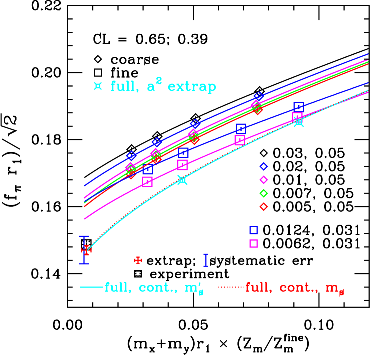
Figure 11: “Pion” decay constants with $m_{x}=m_{y}$ vs. quark mass, in units of $r_{1}$. The relative mass renormalization of coarse and fine lattices has been included so that data from both may be presented on the same plot. Lines come from “Fit B,” a single NNLO fit, Eqs. (33) and (34), to entire data subset II (decay constants and masses). The cyan solid line and red dotted line represent the fit function in “full QCD” (valence and sea masses set equal) after extrapolation of parameters to the continuum. The cyan solid line keeps the $s$ quark mass equal to $m^{\prime}_{s}$ on the fine lattices; while the red dotted line (just barely visible above the cyan solid line) replaces $m^{\prime}_{s}$ with the physical mass $m_{s}$. The cyan fancy squares result from extrapolation of full QCD points to the continuum at fixed quark mass; their agreement with the cyan solid line is a consistency check. Points and fit lines have been corrected for finite volume effects.

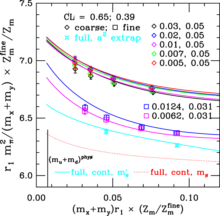
Figure 12: Same as Fig. 11 (Fit B), but squared “pion” masses divided by quark mass are shown. Because taste splittings are smaller for the fine lattices, the average meson mass changes more rapidly with quark mass, and there is greater curvature at small quark mass.

Figures 11 and 12 show our preferred NNLO fit to data subset II. We call this fit “Fit B”; the corresponding fit on data subset I is called “Fit A.” Fit B is a single fit to the data in both Figs. 11 and 12, as well as many more data points not shown. The fit has a chi-square of 192 with 200 degrees of freedom, giving ${\rm CL}=0.65$. This is a standard CL, with $\chi^{2}$ summed over all data points, and number of degrees of freedom (d.o.f.) given by number of data points minus the number of parameters. If we include the Bayesian priors as effective “data points,” then Fit B has a chi-square of 235 with 230 degrees of freedom, CL=0.39. The fact that this is also an acceptable CL indicates that S$\chi$PT and our assumptions about the $a$-dependence of fit parameters are reasonably well behaved in this mass range. Fit A gives very similar results for decay constants and quark masses, but includes many fewer points (94 vs. 240) and has a lower confidence level (0.23). As discussed in Sec. IX.4.4, however, Fits A and B produce rather different values for the low energy constant $2L_{6}-L_{4}$, indicating a large systematic uncertainty in that parameter. For our central values of the $L_{i}$, we average the results of Fit A and B, and include the difference in the error.

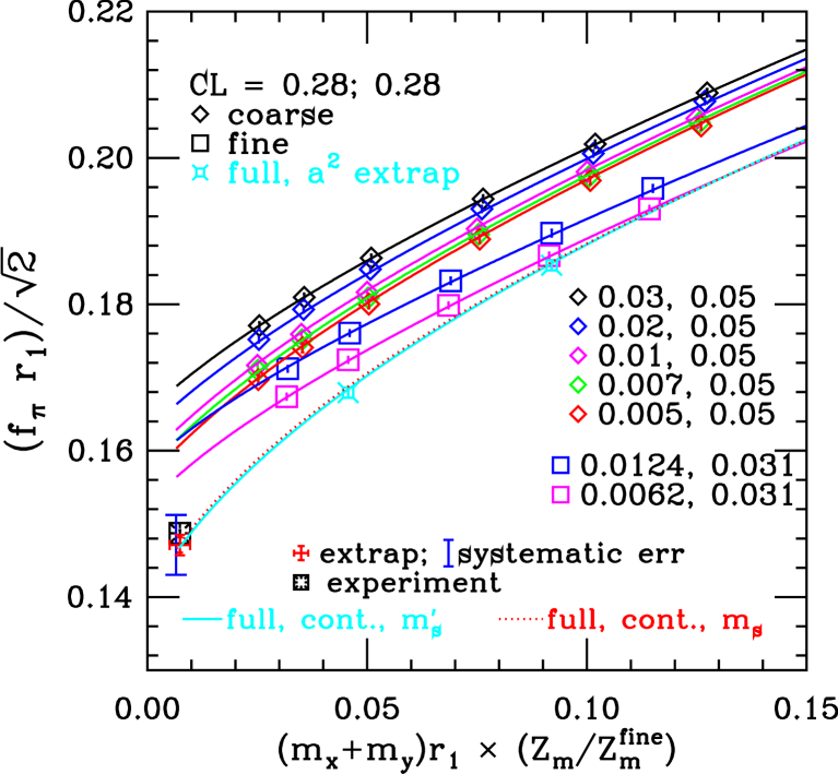
Figure 13: “Pion” decay constants with $m_{x}=m_{y}$ in data subset III. Lines come from Fit C, a single NNNLO fit to masses and decay constants. The cyan solid line, red dotted line, and cyan fancy squares have the same meaning as in Fig. 11. Points (and fit lines) have been corrected for finite volume effects.

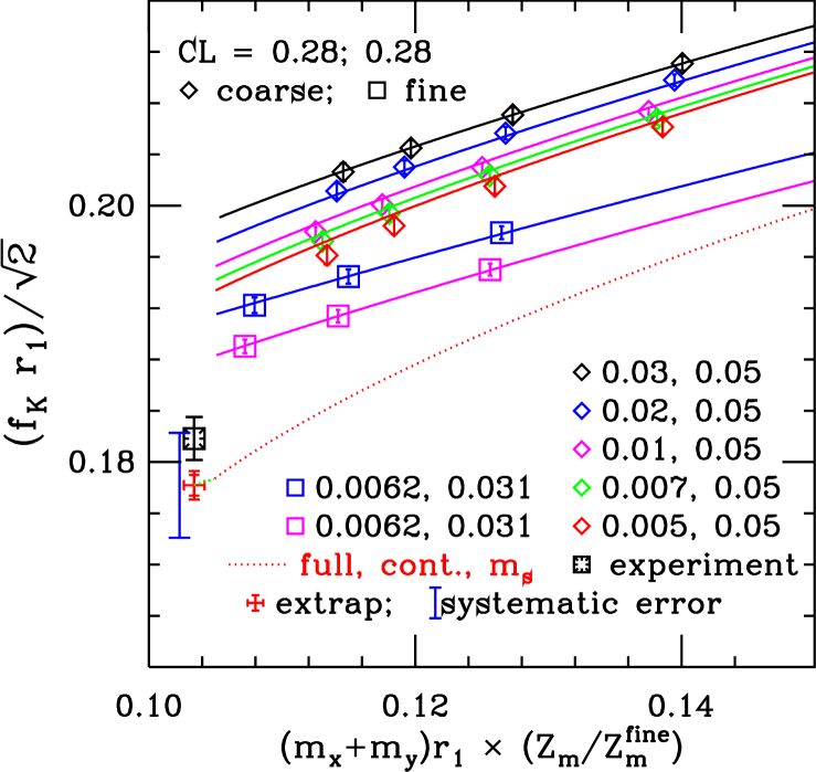
Figure 14: Similar to Fig. 13 (Fit C), but for “kaon” decay constants, with $m_{y}$ fixed as closely as possible on each set to $m_{s}^{\rm phys}$. The red dotted line has parameters extrapolated to the continuum, the strange valence and sea masses set to the physical value, and light sea quark mass equal to light valence mass $m_{x}$. The green dotted extension has the light sea quark mass fixed at $\hat{m}$, and the valence mass $m_{x}$ continuing down to $m_{u}$ (thus giving $f_{K^{+}}$).

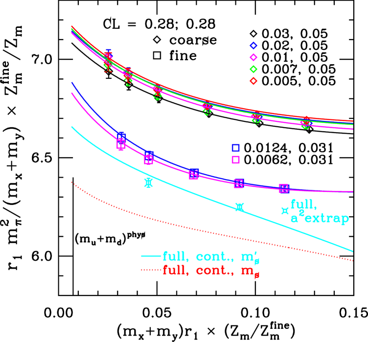
Figure 15: Same as Fig. 13 (Fit C), but for squared “pion” masses divided by quark mass.

Figures 13, 14, and 15 show $\pi$ and $K$ decay constants and $\pi$ masses from the corresponding preferred NNNLO fit to data subset III (“Fit C”). The LO and NLO parameters here are fixed, up to their statistical errors, by Fit B. Fit C has a chi-square of 383 for 368 degrees of freedom (CL=0.28); including the priors gives a chi-square of 418 for 402 degrees of freedom (CL=0.28). Central values of $f_{K}$, $f_{\pi}$, $f_{K}/f_{\pi}$, $m_{s}$, $\hat{m}$, $m_{s}/\hat{m}$, and $m_{u}/m_{d}$ are taken from this fit; while Fits A and B are included as alternatives in estimating systematics.

Using the volume-dependence from NLO S$\chi$PT, Eqs. (13) and (14), the leading finite volume effects can be removed from our data. Such effects are rather small to begin with ($<0.9\%$ on $M^{2}_{P^{+}_{5}}$ and $<1.4\%$ on $f_{P^{+}_{5}}$, based on fit B), and this calculated volume-dependence is consistent with simulation results in the one case where two different volumes are available MILC_SPECTRUM2 . One-loop finite volume effects have been removed from the points and lines shown in Figs. 11 – 15. Possible residual errors from higher order finite volume effects are discussed in Sec. IX.4.6.

To extract continuum results for masses or decay constants from Fits A, B, or C, we first set the taste splitting and the taste violating parameters to zero. We then extrapolate the remaining, physical parameters to the continuum linearly in $\alpha_{S}a^{2}$. For central values, we assume that the ratio of this quantity between fine and coarse lattices is 0.427 (see Eq. (26)). For the LO parameters we take the range of the ratio to be 0.398 to 0.441 in estimating the systematic error, as in the discussion of Eq. (26). But for all other parameters, we expand the range to 0.30 to 0.441 in recognition of the fact that the fits do not distinguish generic discretization errors, ${\cal O}(\alpha_{S}a^{2})$, from taste-violating errors, ${\cal O}(\alpha_{S}^{2}a^{2})$. We thus must include the range discussed following Eq. (10).

Table 4 shows the central values of the continuum extrapolated parameters for Fits A, B, and C. Note that the statistical errors on most of the parameters are quite large. This seems to be a consequence of the “flat directions” in the fitting function, as described in Sec. IX.2: small fluctuations in the data can produce large variations in the parameters. However, because of the correlations among the parameters, the statistical errors of interpolated or extrapolated decay constants and masses are small, comparable to those of the raw data.

	Fit A	Fit B	Fit C
$r_{1}\;\mu$	$\phantom{+}5.579(515)$	$\phantom{+}4.549(387)$	$\phantom{+}4.462(227)$
$r_{1}\;f$	$\phantom{+}0.186(14)$	$\phantom{+}0.185(21)$	$\phantom{+}0.185(15)$
$(2L_{6}-L_{4})\times 10^{3}$	$\phantom{+}0.244(156)$	$\phantom{+}0.705(157)$	$\phantom{+}0.763(89)$
$(2L_{8}-L_{5})\times 10^{3}$	$-0.038(96)$	$-0.330(113)$	$-0.392(76)$
$L_{4}\times 10^{3}$	$\phantom{+}0.178(231)$	$\phantom{+}0.200(340)$	$\phantom{+}0.186(239)$
$L_{5}\times 10^{3}$	$\phantom{+}1.834(247)$	$\phantom{+}1.949(263)$	$\phantom{+}2.054(179)$
$\beta^{(m)}_{1}$	$-0.566(80)$	$-0.279(43)$	$-0.260(79)$
$\beta^{(m)}_{2}$	$-0.314(195)$	$-0.994(193)$	$-1.050(124)$
$\beta^{(m)}_{3}$	$\phantom{+}0.208(36)$	$\phantom{+}0.149(33)$	$\phantom{+}0.145(19)$
$\beta^{(m)}_{4}$	$-0.281(22)$	$-0.150(13)$	$-0.081(9)$
$\beta^{(m)}_{5}$	$\phantom{+}0.554(336)$	$\phantom{+}1.658(367)$	$\phantom{+}1.861(310)$
$\beta^{(f)}_{1}$	$\phantom{+}0.237(62)$	$\phantom{+}0.188(36)$	$\phantom{+}0.257(85)$
$\beta^{(f)}_{2}$	$\phantom{+}0.135(142)$	$\phantom{+}0.131(209)$	$\phantom{+}0.128(141)$
$\beta^{(f)}_{3}$	$\phantom{+}0.189(36)$	$\phantom{+}0.182(33)$	$\phantom{+}0.150(54)$
$\beta^{(f)}_{4}$	$-0.059(36)$	$-0.058(24)$	$-0.062(15)$
$\beta^{(f)}_{5}$	$-0.098(286)$	$-0.115(415)$	$-0.109(389)$
$\sigma^{(m)}$	—	—	$-0.130(44)$
$\rho^{(m)}$	—	—	$\phantom{+}0.049(52)$
$\sigma^{(f)}$	—	—	$-0.063(165)$
$\rho^{(f)}$	—	—	$-0.132(69)$

Table 4: Continuum extrapolated fit parameters for Fits A, B, and C, which are on mass subsets I, II, and III, respectively. No extrapolation errors are included; we show statistical errors only. See Sec. VI for definitions of the parameters.

Once the continuum chiral parameters are obtained, we set valence and sea quark masses equal and obtain “full QCD” formulas for $m^{2}_{\pi}/(2\hat{m}^{\prime})$,  $m^{2}_{K}/(\hat{m}^{\prime}+m^{\prime}_{s})$,   $f_{\pi}$,   and $f_{K}$ in terms of arbitrary quark masses $\hat{m}^{\prime}$ and $m^{\prime}_{s}$. The cyan lines in Figs. 11 – 15 show these as a function of $\hat{m}^{\prime}$, with $m^{\prime}_{s}$ held fixed at the value of the simulation sea quark mass on the fine lattices. As a consistency check, we also show in each case the result from extrapolation of full QCD points to the continuum at fixed quark mass (cyan fancy squares). To generate these points, we use the chiral fits only to interpolate the coarse data so that it corresponds to the same physical quark masses as the fine data. There are just two such points in each plot because we have just two runs with different sea quark masses on the fine lattice. Since discretization errors come both from taste violations and generic errors, there is an ambiguity in the extrapolation used to find these points. We have assumed that taste violations dominate and have extrapolated linearly in $\alpha^{2}a^{2}$, i.e., with a ratio of 0.35 in $\alpha^{2}a^{2}$ between coarse and fine (see discussion following Eq. (10)). This agrees both with our order of magnitude estimates (taste violations $\approx\!6\%$; generic errors $\approx\!2\%$) and with a detailed analysis below (Sec. IX.4.1).

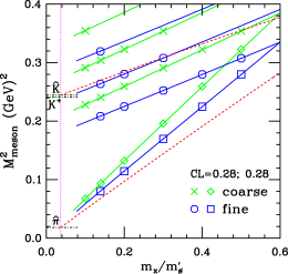
Figure 16: Squared meson masses in subset III, as a function of $m_{x}/m^{\prime}_{s}$. The lines are from Fit C. We show results from two lattices: a coarse lattice with sea quark masses $a\hat{m}^{\prime}=0.01$, $am^{\prime}_{s}=0.05$, and a fine lattice with $a\hat{m}^{\prime}=0.0062$, $am^{\prime}_{s}=0.031$. Three sets of “kaon” points with $m_{y}=m^{\prime}_{s},0.8m^{\prime}_{s},0.6m^{\prime}_{s}$, are plotted for each lattice. “Pion” points have $m_{x}=m_{y}$. The statistical errors in the points are not visible on this scale. The red dashed lines give the continuum-extrapolated fit (now as a function of $m_{x}/m_{s}$), and the magenta vertical dotted line shows the physical $\hat{m}/m_{s}$ obtained. The extension (shown in green ) of the red dashed kaon line until it intersects the QCD $K^{+}$ value then gives $m_{u}/m_{s}$, from which we find $m_{u}/\hat{m}$ or $m_{u}/m_{d}$.

To proceed further we need to know the physical values of the quark masses. These can be obtained from Fig. 12 or Fig. 15 by finding those values of $\hat{m}$ and $m_{s}$ that give the $\pi$ and $K$ their physical QCD masses in the isospin limit, $m_{\hat{\pi}}$ and $m_{\hat{K}}$ (defined in Eq. (VIII)). An iterative procedure is required because both meson masses depend on both quark masses, although the dependence of $m_{\hat{\pi}}$ on $m_{s}$ is mild, since $s$ only appears as a sea quark. The nature of this extrapolation/interpolation is most clearly seen in Fig. 16, which is again Fit C, but now shown for squared meson masses as a function of light quark mass. For clarity, we plot data with only one choice of sea quark masses for the coarse and fine sets; the variation with light sea quark mass is quite small on this scale. The red dashed lines show the fit after extrapolation to the continuum, going to full QCD, and iteratively adjusting the strange quark mass to its physical value, so that the pion and kaon reach their physical QCD values at the same value of $\hat{m}$.

Note that nonlinearities in the data are quite small on the scale of Fig. 16. Linear fits to $m^{2}_{P_{5}^{+}}$ as a function of $m_{x}+m_{y}$ would change the physical quark mass values by only $2\%$ to $7\%$, depending on the range of quark masses included and whether or not we fit the decay constants simultaneously. (The correlation between masses and decay constants implies that the fits are correlated even in this case, where they have no free parameters in common.) However, the tiny statistical errors in our data imply that even small nonlinearities must be accurately represented in order to obtain good fits. Indeed, linear fits have $\chi^{2}/{\rm d.o.f.}\!\sim\!20$. For an example of the accuracy of a linear fit, see the lowest fit line (for Goldstone pions) in Fig. 9.

Once the physical $s$ quark mass $m_{s}$ is in hand, we can adjust the cyan lines in Figs. 11 – 15 to put the strange mass at its physical value. This gives the dotted red lines. Following the dotted red lines to the physical light quark mass $\hat{m}$ gives our extrapolated results for $f_{\pi}$, plotted as red fancy pluses in Figs. 11 and 13. The errors in the red fancy pluses are statistical only; the systematic errors are shown separately. We also plot the “experimental” values of the decay constants PDG , where we put experimental in quotation marks to emphasize that the decay constants are extracted from experiment using theoretical input and values of CKM matrix elements, which themselves have uncertainties.

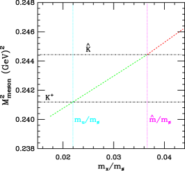
Figure 17: A magnification of the region around the $\hat{K}$ and $K^{+}_{\rm QCD}$ masses in Fig. 16. The dotted vertical lines give $m_{u}/m_{s}$ and $\hat{m}/m_{s}$.

Figure 16, also shows how $m_{u}$ is extracted: With $m_{s}$ and $\hat{m}$ determined, we can continue the full QCD kaon line as a function of the light valence quark mass (holding the light sea quark mass fixed at $\hat{m}$) until it reaches the value of $(m^{2}_{K^{+}})_{\rm QCD}$, Eq. (47). The continuation is shown as a green dashed line. For clarity, a magnified version of the relevant region is shown in Fig. 17. There is a slight change in the slope of the dashed line at $m^{2}_{\hat{K}}$ because, below this mass (green section), the light sea quark mass is no longer changing. Above this point, light valence and sea masses change together. The ratio of the $x$ coordinates of the points where the kaon line intersects the physical $(m^{2}_{K^{+}})_{\rm QCD}$ and $m^{2}_{\hat{K}}$ values is $m_{u}/\hat{m}=0.60$.

Given $m_{u}$, we can extract $f_{K}$, which is really $f_{K^{+}}$, not the decay constant “$f_{\hat{K}}$” of an isospin-averaged kaon. After extrapolating the chiral parameters to the continuum, we set valence and sea strange quark masses equal to the physical $m_{s}$. We now make a two-step extrapolation in the light quark mass, as shown in Fig. 14. We first set the light sea mass equal to the light valence mass $m_{x}$ and extrapolate in $m_{x}$ down to $\hat{m}$ (red dotted line). We then fix the sea quark mass at $\hat{m}$ and continue the extrapolation in valence mass $m_{x}$ to $m_{u}$ (short green dotted line). It is clear from the size of the systematic errors that this final short extrapolation does not at present produce a significant change in $f_{K}$. However, this distinction between $f_{K^{+}}$ and $f_{\hat{K}}$ will become more important as lattice computations improve.

IX.4 Discussion

Good fits are not possible without the taste-violating terms in S$\chi$PT. Figure 10 corresponds exactly to Fig. 11 except that in Fig. 10 the taste splittings in meson masses have been set to zero and the taste-violating chiral parameters ($\delta^{\prime}_{V}$, $\delta^{\prime}_{A}$, $L^{\prime}$, and $L^{\prime\prime}$) have been eliminated. Thus the fit in Fig. 10 is to the “continuum” NNLO $\chi$PT form, which has only four fewer parameters than the S$\chi$PT fit in Fig. 11 (i.e., a total of 36). We put “continuum” in quotation marks here because generic variations in physical parameters between coarse and fine lattices are still allowed. Further, even if we allow these generic variations to be arbitrarily large, instead of the $\approx 2\%$ variation permitted in the standard fits, we cannot obtain good fits without including the taste violations. The fact that continuum $\chi$PT fits are so poor reassures us that the good fit in Fig. 11 is not simply a trivial consequence of having a lot of fit parameters — one has to get the physics right. Other test fits described below, such as fitting without the nonanalytic terms in the fit function (Sec. IX.4.2), give additional reassurance, since they have equal or comparable numbers of parameters to Fit B but cannot describe the lattice data.

IX.4.1 Continuum extrapolation

For the decay constants, our preferred method of continuum extrapolation is to extrapolate the chiral fit parameters, as described in Sec. IX.3. An alternative method is to determine decay constants in physical units at fixed lattice spacing, and then attempt to extrapolate these quantities. There are two ways to find fixed lattice-spacing values: (1) simply use the complete chiral fits to extract the decay constants on the coarse or fine sets, or (2) first set the taste-violating parameters ($\delta^{\prime}_{V}$, $\delta^{\prime}_{A}$, $L^{\prime}$, $L^{\prime\prime}$) and splittings in the fit to zero, and then extract the decay constants for each set. The advantage of method (2) is that, once taste-violations have been set to zero, remaining discretization errors should be dominantly of the generic type, so we may extrapolate to the continuum linearly in $\alpha_{S}a^{2}$. In method (1), the decay constants at fixed $a$ have both generic and taste-violating discretization errors, so there is an ambiguity in extrapolating them to the continuum.

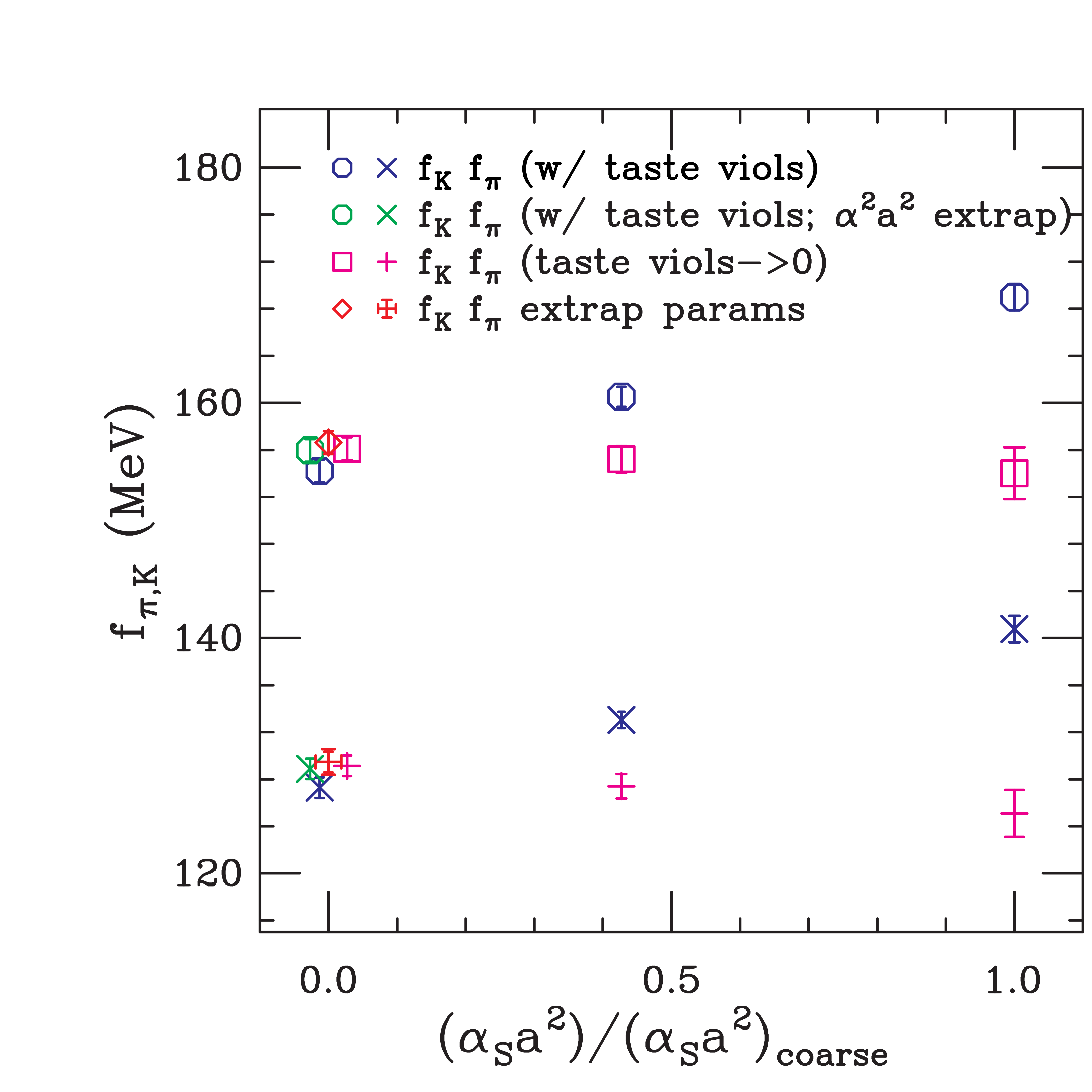
Figure 18: Dependence of chirally-extrapolated $f_{\pi}$ and $f_{K}$ on lattice spacing. The blue octagons and crosses show values at fixed lattice spacing (using “method (1)”) and those extrapolated to the continuum linearly in $\alpha a^{2}$. For the green octagons and crosses, the extrapolation is linear in $\alpha^{2}a^{2}$. The magenta squares and pluses have the taste-violating effects at fixed lattice spacing removed with S$\chi$PT (“method (2)”); the points are then extrapolated to the continuum linearly in $\alpha a^{2}$. The red diamond and fancy plus are the results of extrapolating the chiral fit parameters to the continuum. Extrapolated points at $a=0$ have been moved slightly horizontally for clarity. Fit C is used everywhere.

Figure 18 shows the decay constants at fixed $a$ using both methods, and the various extrapolations to the continuum. Once taste violations are removed (method (2)), the remaining discretization errors are quite small, giving a $1\%$–$2\%$ change between coarse and fine, as expected. Further, because this change is small, it would not make a significant difference in the extrapolated answer if we were to replace the $\alpha_{S}a^{2}$ extrapolation with an $\alpha^{2}_{S}a^{2}$ one. With method (1), the change from coarse to fine is $5\%$–$6\%$, roughly the same size as the difference in the raw data between these lattices: See Figs. 11 – 15. There is also a noticeable difference ($\approx\!1.2\%$) in the extrapolated results with method (1), depending on whether ${\cal O}(\alpha_{S}a^{2})$ or ${\cal O}(\alpha^{2}_{S}a^{2})$ errors are assumed. This ambiguity would grow to $\approx\!2.2\%$ if we used the full allowed range of values for the ${\cal O}(\alpha_{S}a^{2})$ or ${\cal O}(\alpha^{2}_{S}a^{2})$. For $f_{\pi}$ and $f_{K}$, we therefore do not consider method (1) results among the possible alternatives in assessing the systematic error. We use the parameter-extrapolated version (red diamond and fancy plus in Fig. 18) for central values, and include the results of method (2) when estimating systematic errors. Note that we are rejecting method (1) because of its inherent ambiguity, not because it disagrees with the other methods of extrapolation.

On the other hand, for the ratio $f_{K}/f_{\pi}$ and for quark masses ($m_{u}/m_{d}$ here, and $m_{s}$, $\hat{m}$ and $m_{s}/\hat{m}$ in Ref. strange-mass ), the results change little with lattice spacing, so the ambiguity in method (1) is tiny (much less than other systematic errors). Therefore, in those cases we include all three methods of extrapolation in our systematic error estimates.

The nice consistency of Fig. 18 with our understanding of the sources of discretization errors is comforting. However, we caution the reader that some aspects of this picture are dependent on the assumptions that went into our fits. In particular, we have inserted Bayesian priors to enforce a (1 standard deviation) constraint that LO chiral parameters change by at most $2\%$ from coarse to fine lattices. When we relax this constraint to $4\%$, the difference of method (2) results from coarse to fine increases to $3\%$–$4\%$; while method (1) differences remain at about $6\%$. The relaxed version of the chiral fit is included in the systematic error analysis. With just two lattice spacings, however, we cannot remove this constraint entirely without the fit becoming unstable, as has been emphasized in Sec. IX.2. Instead, the key point here is that we can obtain good fits of our entire data set based on the theory of taste violations, plus some smaller generic errors. This is to be contrasted with our failed attempts to fit the data without including taste-violations, even when generic errors are allowed to be arbitrarily large.

IX.4.2 Evidence for chiral logarithms

From Sec. VI.2, we know that the coefficient of the chiral logarithm terms, the chiral coupling $1/(16\pi^{2}f^{2})$, is not tightly constrained by the fits. If the chiral coupling is allowed to be a free parameter, fits to higher valence masses prefer values of $f$ near $f_{K}$ in the coupling; while fits to lower masses prefer $f$ closer to $f_{\pi}$. On the other hand, acceptable fits can be obtained for all our mass ranges with the chiral coupling fixed anywhere between its value for $f_{\pi}$ and that for $f_{K}$. Given this freedom, can we claim that chiral logarithms are observed at all? To answer this question, we consider a variety of alternative fits without chiral logarithms.

First of all, since Fig. 16 appears so linear to the eye, one can ask whether a simple linear fit would work. The answer is no: linear fits of $m^{2}_{P_{5}^{+}}$ vs. $m_{x}+m_{y}$ have chi-square per degree of freedom $\sim\!20$. The point is that the statistical errors in the data are so small, and the correlations are well enough determined, that the small departures from linearity must be accurately represented by the fits. These deviations are seen more clearly in Figs. 12 and 15, where the valence quark masses are divided out. Similarly, even though the apparent curvature in the decay constant data is not large (see Figs. 11 and 13), linear fits of $f_{P^{+}_{5}}$ vs. $m_{x}+m_{y}$ are also terrible, with chi-square per degree of freedom $\sim\!25$.

We next check whether the data can be fit by including all the higher order (non-linear) analytic terms, but omitting the chiral logarithms. With the chiral logarithm functions $\ell$, Eq. (13), and $\tilde{\ell}$, Eq. (14), set to zero, we attempt a fit directly comparable to our NNLO Fit B on mass subset II. This fit has 38 free parameters, which is 2 less than Fit B because the taste-violating hairpin parameters $\delta^{\prime}_{A}$ and $\delta^{\prime}_{V}$ decouple when $\ell=\tilde{\ell}=0$. Despite the large number of parameters, the fit is very bad, with $\chi^{2}/{\rm d.o.f.}=7.38$ for 202 degrees of freedom; ${\rm CL}<10^{-194}$.

Bećirević and Villadoro Becirevic:2003wk , have pointed out that, for some current simulations on small volumes, the finite size effects are much more important than the actual chiral logarithms. We would not expect that to be the case here since the lattice volumes are relatively large ($L\geq 2.5\;{\rm fm}$) and finite volume effects here are small (at most 1.4% — see Sec. IX.3). To check this expectation, we first removed the finite volume effects from the data using Fit B, and then fit again to the 38 parameter form with $\ell=\tilde{\ell}=0$. This fit is improved over the previous one, but still quite bad: $\chi^{2}/{\rm d.o.f.}=3.08$ for 202 degrees of freedom; ${\rm CL}<10^{-43}$. Our conclusion is that the effect of the staggered chiral logarithms is in fact observed in our data.

One can ask whether the finite volume effects are also directly observed. The answer seems to be yes: A 40-parameter fit leaving out these effects (setting $\delta_{1}$ and $\delta_{3}$ to zero in Eqs. (13) and (14)) but otherwise identical to Fit B has $\chi^{2}/{\rm d.o.f.}=1.95$ for 200 degrees of freedom; ${\rm CL}\approx 2\times 10^{-14}$.

IX.4.3 Are the lattice masses light enough for S$\chi$PT to be applicable?

To discuss this question, we first have to say what we mean by the physical quark masses at fixed $a$. For current purposes we define the physical values of the lattice masses, $am_{s}$ and $a\hat{m}$, by method (2), i.e., as the quark masses that give the pion and kaon their physical masses when all taste splittings and taste-violating chiral parameters are set to zero. This gives $am_{s}\approx 0.0457$, $a\hat{m}\approx 0.00166$ on the coarse lattices and $am_{s}\approx 0.0289$, $a\hat{m}\approx 0.00105$ on the fine. We have not made a detailed study of the errors in these numbers, but systematic errors are $\sim\!6\%$, and statistical errors are 1% or less. We could alternatively define the physical $m_{s}$ at a given lattice spacing by method (1), i.e., as the masses that give the physical mesons masses directly, including all effects of taste violations in the chiral loops. The latter values of quark masses were quoted in strange-mass ; MILC_SPECTRUM2 and are about $\sim\!15\%$ smaller on the coarse lattices and $\sim 6\%$ smaller on the fine lattices than the ones quoted above. We choose the method (2) definition here because we are going to be adding on the taste-splittings to meson masses explicitly. We note that the difference between the methods becomes becomes small, $1\%$–$2\%$, once we extrapolate to the continuum, and is included in the systematic errors quoted in Ref. strange-mass .

We now consider meson masses on the coarse lattice for subset II. This is the worst case because subset II contains the highest valence quark masses for which we have applied a fully chiral description, and the coarse lattices have the largest additional contributions to meson masses from taste violations. The valence masses here obey $m_{x}+m_{y}\leq 0.7m^{\prime}_{s}\approx 0.77\,m_{s}$. Since the smallest valence mass is $0.1\,m^{\prime}_{s}$, the largest is $0.6\,m^{\prime}_{s}\approx 0.66\,m_{s}$; while the largest sea quark mass in the simulation is $m^{\prime}_{s}\approx 1.09\,m_{s}$. For the following estimates, we assume linear dependence of squared meson masses on quark masses, and take $486\,{\rm Me\!V}$ as the mass a “kaon” would have in the absence of electromagnetism and if the light quark were massless. In other words, we use $\mu m_{s}=(486\,{\rm Me\!V})^{2}$. This comes from Eq. (VIII) and the ratio $m_{s}/\hat{m}=27.4$ strange-mass . Then the largest valence-valence Goldstone meson mass in coarse subset II is $425\,{\rm Me\!V}$. Adding on the largest splitting (the taste-singlet case) gives $623\,{\rm Me\!V}$; while an “average” taste splitting (see discussion after Eq. (12)) gives $551\,{\rm Me\!V}$. We do not think it unreasonable to expect S$\chi$PT to work in this mass range, although it is not surprising — considering the small statistical errors of the data — that NNLO terms are needed. Further, the comparison with subset I results is a good check, because the corresponding masses there are significantly lower: $321\,{\rm Me\!V}$, $557\,{\rm Me\!V}$, and $475\,{\rm Me\!V}$, respectively.

Mesons with one or two sea quarks also appear in chiral loops. These are generally comparable to the masses just discussed. But they are significantly larger when the sea quark is an $s$, which is exacerbated by the fact that the simulation value, $m^{\prime}_{s}$, is larger than the physical mass. On subset II, this largest valence-sea (Goldstone) mass is $642\,{\rm Me\!V}$. Adding on the biggest splitting gives $787\,{\rm Me\!V}$. This taste-singlet meson enters with a factor $1/16$ in the sum over tastes; the “average” taste version is $731\,{\rm Me\!V}$. On subset I, the masses become $578\,{\rm Me\!V}$, $736\,{\rm Me\!V}$, and $676\,{\rm Me\!V}$, respectively. Further, there are sea-sea contributions, which are independent of the valence mass subset. The most relevant here is the taste-singlet $\eta$. Its mass depends (mildly) on the light quark sea masses, but is $\sim\!765\;{\rm Me\!V}$ including splitting. In addition there are $\eta^{\prime}$-like particles in the taste axial and vector channels whose masses are comparable to the taste-singlet $\eta$ but have smaller (${\cal O}(a^{2})$) couplings.

The meson masses involving the $s$ sea quark are admittedly quite high to expect that even NNLO $\chi$PT will be accurate. For example, the largest mass mentioned above, $765\;{\rm Me\!V}$, corresponds to a $\chi_{q}$ value, Eq. (11), of 0.43. This suggests an error from neglected terms of order $(0.43)^{3}=8\%$. But, just as for the valence subset III, the issue here for decay constants and quark masses is only to get a good interpolation to the physical $s$ quark mass. Indeed, if the $s$ sea quark in the simulation had been chosen at the a posteriori determined physical mass, we would not have needed to use $\chi$PT for the $s$ at all, but could use a $SU_{L}(2)\times SU_{R}(2)$ $\chi$PT for the light quark extrapolation. The systematic error on the coarse lattice from adjusting $m^{\prime}_{s}=1.09m_{s}$ to $m_{s}$ may be crudely estimated as $(0.43)^{3}\times[(1.09)^{3}-1]\approx 2\%$. Since $m^{\prime}_{s}$ is closer to $m_{s}$ on the fine lattice, some of this error will be extrapolated away when we go to the continuum limit. On the other hand, chiral coefficients (at NLO and NNLO) that involve the sea quarks are not fit accurately because the “lever arm” is small: the sum of the sea quark masses changes by less than a factor of 2 over our entire range of coarse lattices and only by 30% for the fine lattices. A more reliable estimate of the error in adjusting the $s$ quark mass comes from considering the range in results over the full list of alternative mass subsets, chiral fits, and continuum extrapolations. It can be as large as half the total chiral error in our results for decay constants and quark masses (see line a1 in Tables 5 and 6); the remaining error comes from extrapolating in the light quark mass.

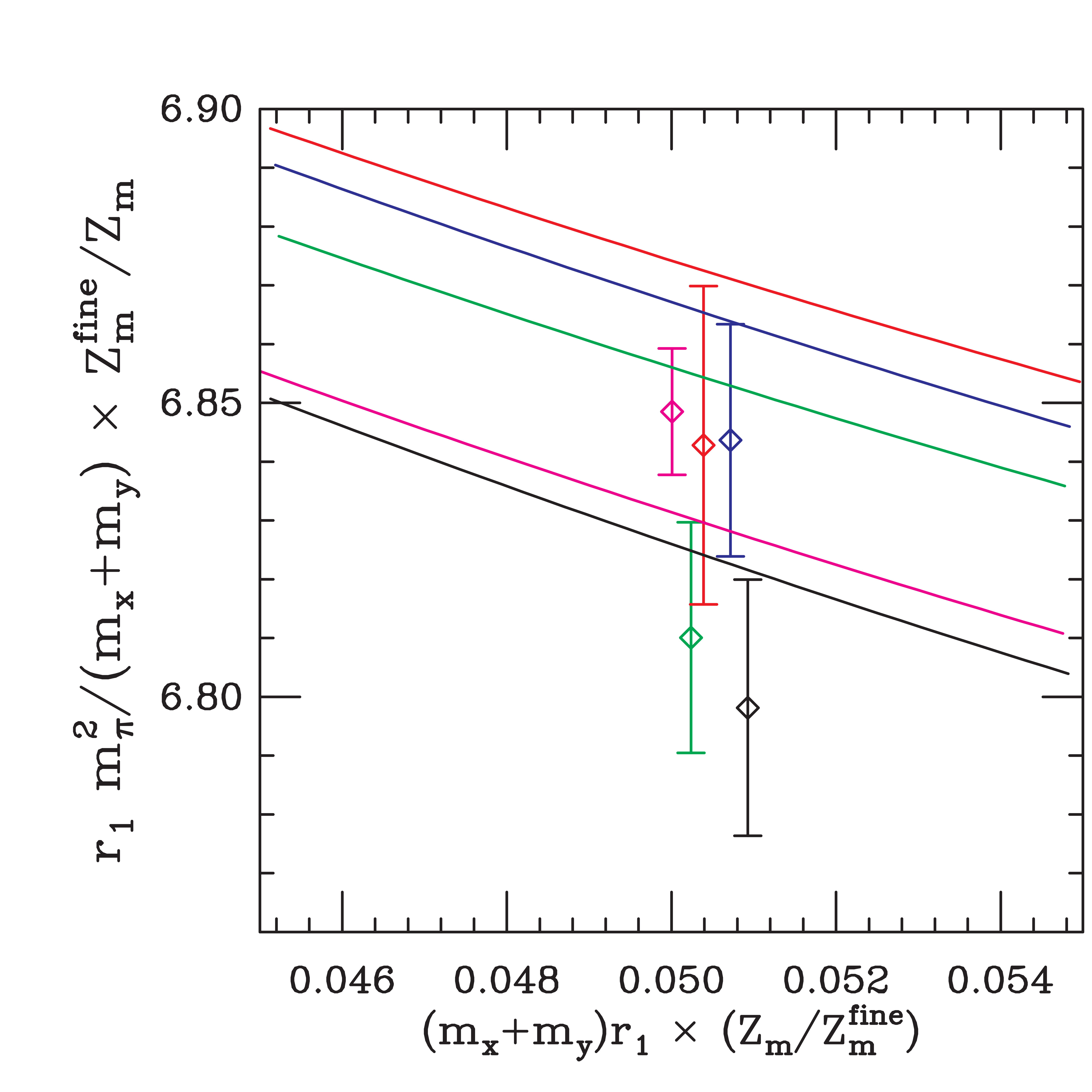
Figure 19: Enlargement of a small region of Fig. 12.

For the $L_{i}$, the situation is somewhat different. Missing higher order terms in the $SU_{L}(3)\times SU_{R}(3)$ expansion mean that there is spurious analytic dependence on the light quark masses that increases as meson masses get larger. Here we are missing the NNLO chiral logarithms, so those terms determine the size of the errors. Letting $M$ be a generic meson mass, the absent terms are of order $M^{4}\log(M^{2})/(8\pi^{2}f_{\pi}^{2})^{2}$. Putting in the largest meson masses discussed above, results in an estimate of the absolute error in the $L_{i}$ of a few times $10^{-4}$. This is indeed the size of the errors we observe when we consider all the alternative chiral fits discussed above and/or restrict the valence masses to subset I instead of subset II (Sec. X). The low energy constant $2L_{6}-L_{4}$ may be an exception: Since the errors in it are large on this scale, $\sim\!4\times 10^{-4}$, they may also not be very reliable. Difficulty in extracting $2L_{6}-L_{4}$ is again related to the small lever arm for the sea quark dependence. This can be seen in Fig. 19, an enlargement of a small region of Fig. 12. As the sea quark mass is changed, the differences are small — comparable to statistical errors — and not monotonic. Contrast this with the monotonic sea quark dependence seen for $f_{\pi}$ in Fig. 11. A coarse simulation now in progress, with all three sea quark masses at about $0.66m_{s}$, should help to reduce significantly the error in the sea quark mass dependence.

IX.4.4 Convergence of $\chi$PT

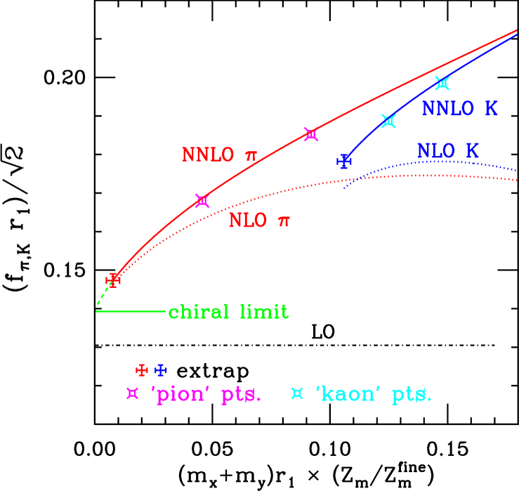
Figure 20: Convergence of $SU(3)_{L}\times SU(3)_{R}$ $\chi$PT for decay constants. Our results on mass set II for $f_{\pi}$ and $f_{K}$ at LO (dash-dotted black line), NLO (dotted red and blue curves), and NNLO (solid red and blue curves) are shown. The chiral parameters have been extrapolated to the continuum. Convergence of $SU(2)_{L}\times SU(2)_{R}$ $\chi$PT  can be seen by comparing the $f_{\pi}$ results to the chiral limit, obtained (green dashed curve) by extrapolating the NNLO $f_{\pi}$ result to $\hat{m}=0$. The magenta and cyan fancy squares are found by extrapolating our full QCD data to the continuum limit at fixed quark mass. All results come from Fit B.

Figure 20 shows the convergence of $SU(3)_{L}\times SU(3)_{R}$ $\chi$PT for $f_{\pi}$ and $f_{K}$. All chiral parameters in this plot have been extrapolated to the continuum. The NLO terms contribute $\!20\%$. This is true even for $f_{\pi}$, because $m_{s}$ does not vanish in the chiral limit. The convergence of $SU(2)_{L}\times SU(2)_{R}$ $\chi$PT for $f_{\pi}$ can also be extracted from this plot by starting with the “chiral limit” line instead of the “LO” line lowest order contribution to $f_{\pi}$. Note that the magenta and cyan fancy squares, which are included as a consistency check, are the only full QCD points that we can extrapolate to the continuum at fixed mass. We have lighter valence quarks on the fine lattices, and lighter valence and sea quarks on the coarse lattices. All such partially quenched points are included in the fits that produce the lines in the plot. Figure 20 comes from the fit to data subset II (Fit B). If instead we restrict the fit to data subset I (Fit A), the picture is virtually unchanged.

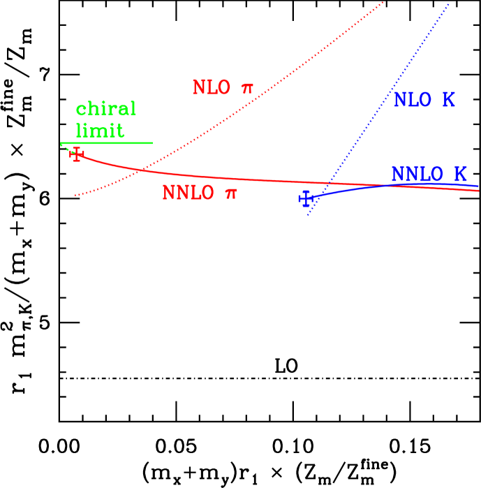
Figure 21: Same as Fig. 20, but for $m_{P+}^{2}/(m_{x}+m_{y})$. This uses Fit B (data subset II).

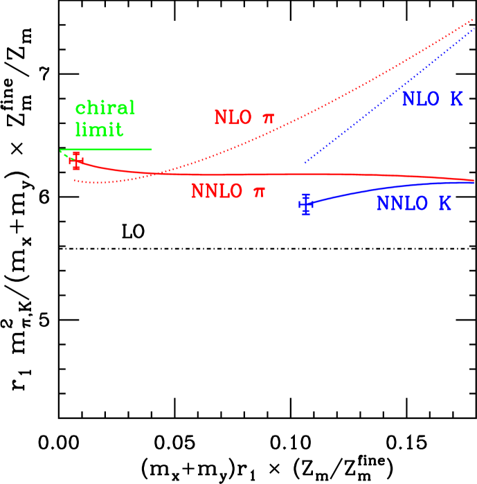
Figure 22: Same as Fig. 21, but for Fit A (data subset I).

Figures 21 and 22 are the corresponding plots for meson masses ($m^{2}_{P^{+}}/(m_{x}+m_{y})$). Figure 21 is generated from the fit to data subset II (Fit B); while Fig. 22 uses data subset I (Fit A). Here there is a significant difference between the two plots, with the latter showing much smaller higher order corrections in $SU(3)_{L}\times SU(3)_{R}$ $\chi$PT than the former. The difference illustrates the poor control over the low energy constant $2L_{6}-L_{4}$ (see Sec. IX.4.3): We get $2L_{6}-L_{4}=0.70(17)\times 10^{-3}$ with Fit B, and $2L_{6}-L_{4}=0.24(16)\times 10^{-3}$ with Fit A. Because this parameter multiplies $2\hat{m}+m_{s}$, its effect does not vanish in the chiral limit of the light quark mass $\hat{m}$. Its variation is largely canceled by differences in the LO parameter $\mu$ and the NNLO parameters $\beta_{2}^{(m)}$ and $\beta_{5}^{(5)}$, Eq. (33), so that the full NNLO fit line and the extrapolated $\pi$ and $K$ values are quite close in the two fits. This means that the ambiguity in $2L_{6}-L_{4}$ and the LO term is largely irrelevant to the extraction of quark masses (and, indirectly, decay constants); the variation between the fits is of course included in systematic errors estimates of these quantities.

The qualitative expectation from $\chi$PT is that coefficients in the expansion should be ${\cal O}(1)$ when we use the dimensionless expansion parameters $\chi_{q}$, Eq. (11). Both Fit A and Fit B pass this test (the largest coefficient in either is $\beta^{(m)}_{2}\approx 1.66$ in Fit B — see Table 4), so we must accept the large systematic effect on $2L_{6}-L_{4}$ as inherent in the current data set. Indeed, the size of the difference in the LO term, $\mu$, between the two fits is reasonable, given that the fits prefer a chiral coupling $1/(16\pi^{2}f^{2})$ with $f$ moving from $\approx\!f_{\pi}$ to $\approx\!f_{K}$ as the quark masses rise toward $m_{s}$ (see comments about the parameter $\omega$ in Sec. VI.2). Both fits here fix $f=f_{\pi}$, but Fit B is effectively able to reduce the effect of the chiral coupling by reducing the LO parameter $\mu$ and compensating by increasing the NLO parameter $2L_{6}-L_{4}$. Since the difference between $f^{2}_{\pi}$ and $f_{K}^{2}$ is more than $40\%$, the $\sim\!20\%$ difference between the $\mu$ from the two fits is not unexpected. New simulations with lighter strange sea quark masses will allow us to take all quark masses deeper into the chiral regime, as well as greatly increase the lever arm on the $m_{s}$ dependence, and should help to resolve this issue.

IX.4.5 Mass dependence of renormalization scheme

Strictly speaking, it is incorrect to use a scale determined by a quantity like $r_{1}$ or the $\Upsilon^{\prime}$–$\Upsilon$ mass difference in chiral fits to lattice data, since such quantities themselves have some (small) sea quark mass dependence not included in chiral perturbation theory Sommer:2003ne . We have investigated this effect by changing to a mass-independent renormalization scheme: Instead of fixing the (relative) lattice scale for particular sea quark mass values from $r_{1}/a$ at those values, we can use, on each lattice, the value of $r_{1}/a$ after extrapolation to the physical mass values using the fit Eq. (7). This produces the same value of $a$ on all the coarse (or, separately, fine) lattices, independent of the sea quark masses. We include the difference between the mass independent scheme and our standard approach in our assessment of systematic errors.

For decay constants and quark masses, the change in scheme is a priori unlikely to make much difference because the physical point is unaffected — all that may change is the extrapolation to it. Further, any low-order analytic dependence on sea quark mass introduced though $r_{1}$ would automatically be compensated by changes in the analytic chiral fit parameters. So the only problem would be due to nonanalytic quark mass dependence, which is probably quite small because $r_{1}$ is a short-distance quantity, at or near the perturbative region. We thus consider the variation in scheme simply as another alternative version of the chiral fits. This means that it would affect the final systematic error only if it produced the largest difference from the central value over all the alternatives. In fact it is fairly small, as expected (see line a3 in Tables 5 and 6).

The situation is logically quite different for the low energy constants. Here, analytic sea quark mass dependence in $r_{1}$ would directly change the output values of $L_{4}$ and $2L_{6}-L_{4}$, which multiply sea quark masses. We therefore consider the scheme dependence as a systematic error in its own right, and add any error found in quadrature with other systematic errors. In practice, however, this effect is still smaller than other errors (see Table 7).

IX.4.6 Residual finite volume effects

At the precision we are working (especially for $f_{K}/f_{\pi}$), it is important to consider whether finite volume effects coming from terms beyond one-loop in S$\chi$PT could be non-negligible. Indeed, Colangelo and Haefeli Colangelo:2004xr have recently investigated such effects in full continuum QCD. For volumes and masses comparable to those used here, they find large higher order corrections to the volume dependence, roughly 30% to 50% of the one-loop results.

In asymptotically large volumes, the finite-volume effects in S$\chi$PT are suppressed relative to those in continuum $\chi$PT for the same (Goldstone) masses because most of the pions entering chiral loops have larger masses. This can be easily seen in Eq. (24): the lightest (Goldstone) pion appears with a weight 1/16 as large as in the continuum. However, at our current volumes, masses, and lattice spacings, the relation between S$\chi$PT and $\chi$PT finite volume effects is complicated, with the former just as likely to be larger than the latter as smaller. Equations (24) and (VI.1), together with our numerical results for splittings (Table 3) and the taste-violating hairpin parameters (Eq. (IX.4.8), below), show how the asymptotic rule can be violated. Since $\Delta_{A}$ is the smallest splitting, and $\delta^{\prime}_{A}$ is non-negligible and negative, $m_{\eta^{\prime}_{A}}$ may not be much larger than the Goldstone pion mass. Then, due to the factors of 4 in Eq. (24), finite volume corrections coming from the $\eta^{\prime}_{A}$ can be as large or larger than the continuum corrections. As $a\to 0$, the term $\ell(m^{2}_{\eta^{\prime}_{A}})$ would be canceled by $\ell(m^{2}_{\pi_{A}})$, but this cancellation may not be effective for finite volume effects at a given value of $a$, because the volume effects are sensitive to small mass differences. Since one-loop finite volume effects on our lattices are comparable to those in the continuum, we have no a priori reason to expect that our results are protected from the higher order effects Colangelo:2004xr seen in the continuum.

Assuming that the higher order finite volume effects in S$\chi$PT are roughly the same size as those in full continuum QCD when the volumes and the masses of the mesons in the loops are the same, we can estimate the resulting systematic errors. For our data, the biggest one-loop finite volume effects appear when both the valence masses and $\hat{m}^{\prime}$ are small (giving a light $\eta^{\prime}_{A}$ in the two-flavor case, Eq. (VI.1), or a light $\eta_{A}$ in the three flavor case, Eq. (VI.1)). The worst case occurs in the coarse run with $a\hat{m}^{\prime}=0.007$; the run with $\hat{m}^{\prime}=0.005$ has smaller finite volume effects because $L\approx 3.0\;$fm there, instead of $L\approx 2.5\;$fm for other runs. From the calculations in Ref. Colangelo:2004xr , we estimate that the residual higher order finite volume effect is at most $0.47\%$ in $f_{\pi}$, $0.24\%$ in $f_{K}$, and $0.23\%$ in $f_{K}/f_{\pi}$. More stringent bounds on the errors can be obtained by removing from the data set those points that have the largest finite volume corrections. Eliminating 8 of 240 points from mass subset II (5 from coarse run $0.007/0.05$, 2 from coarse run $0.01/0.05$, and 1 from fine run $0.0062/0.031$), we lower the largest one-loop finite volume effect on $f_{P^{+}_{5}}$ or $M^{2}_{P^{+}_{5}}$ from $1.35\%$ to $0.81\%$. Not surprisingly, since the reduced data set retains most of the lowest valence mass points and all of the lowest sea mass points, it produces nearly identical results (within $0.05\%$) as the original set. But a repeat of the analysis using Ref. Colangelo:2004xr now bounds the residual finite volume error by $0.29\%$ in $f_{\pi}$, $0.15\%$ in $f_{K}$, and $0.14\%$ in $f_{K}/f_{\pi}$. These are negligible compared to our other systematic errors. In the future, however, as quark masses in staggered simulations decrease further, it will be necessary either to have a better handle on these higher order effects in S$\chi$PT or to go to significantly larger volumes.

IX.4.7 Fourth root of the determinant

In order to eliminate the quark doubling that is still present in the staggered action, the simulations here take the fourth root of the quark determinant for each flavor in order to reduce the quark tastes from 4 to 1 per flavor. There is apparently no ultra-local lattice action that would correspond to the effective action that results from taking this fourth root. The possibility thus exists that physical non-localities will remain in the continuum limit, potentially spoiling the description of QCD by the staggered action. The good agreement of the staggered results with experiment and with continuum chiral behavior plus understood discretization effects (both in current and previous work BIG_PRL ; MILC_SPECTRUM2 ; MASON_ALPHA ) lead us to believe that this is not a problem, but the question is not settled.

The comparison of simulation data with S$\chi$PT forms allows us to make a crude but somewhat more direct test of the fourth root trick. Equations (17) and (18), as written, take into account the fourth root by dividing each sea quark loop contribution by 4, to leave 1 taste per flavor. It is a simple exercise to generalize Eqs. (17) and (18) to make the number of tastes remaining a free parameter. We can then ask what number of tastes per flavor is preferred by the simulation data. With a fit otherwise identical to our standard NNLO fit, we find $1.44(15)$ for the preferred number of tastes per flavor on data subset II, and $1.28(12)$ on the lighter masses in subset I, where the errors are statistical only. If we allow the chiral coupling to vary also (choice (3) fits, Sec. VI.2), we get $1.35(18)$ and $1.22(14)$ on subsets II and I, respectively. In the latter case, the coefficient $\omega$ corresponds to an $f$ in the chiral coupling that is about halfway between $f_{\pi}$ and $f_{K}$ ($\omega\approx 0.82(11)$), which is reasonable. Given that the fits in any case do not tightly constrain the chiral logarithm terms (see Sec. VI.2), we consider these results satisfactory.

We note that there has been recent numerical NUMERICAL and analytic ADAMS work indicating even more directly that the fourth root trick should work as expected. On the other hand, there have been two other recent papers that purport to show problems with locality NONLOCAL . We do not believe the latter work is worrisome because it does not take into account the taste structure of staggered quarks. Instead of trying to project onto a single taste to find the fourth root of the determinant, those papers look only at the fourth root of the Dirac operator itself. That procedure, in our opinion, is almost guaranteed to find a nonlocal result, just as it would in trying to reduce eight Wilson fermions to two, which certainly has an alternative, local solution.

IX.4.8 Taste violating hairpins

Before turning to our physical results, we quote the values of the two taste-violating hairpin parameters coming from the fits. Together with the splittings, Table 3, these parameters appear in S$\chi$PT calculations for other physical quantities, such as heavy-light decay constants CA_CB3 . Averaging values from Fits A and B, we find, on the coarse lattices:

$$r_{1}^{2}a^{2}\delta^{\prime}_{A} = -0.28(3)(5)$$

$$r_{1}^{2}a^{2}\delta^{\prime}_{V} = -0.11(8)({}^{+21}_{-4})\ ,$$ (48)

where the errors are statistical and systematic, respectively. The latter error comes from the variation over all acceptable chiral fits on mass subsets I and II. The parameter $a^{2}\delta^{\prime}_{A}$ is comparable in size to the taste-violating splittings (Table 3); while $a^{2}\delta^{\prime}_{V}$ is consistent with zero but poorly determined. The values of $a^{2}\delta^{\prime}_{A}$ and $a^{2}\delta^{\prime}_{V}$ on the fine lattices are not fit separately but are constrained to be 0.35 times as large for central-value fits. (See discussion following Eq. (10).)

X Final Results and Conclusions

The central values and error estimates for $f_{\pi}$, $f_{K}$, and $f_{K}/f_{\pi}$ are collected in Table 5. Central values come from Fit C (mass subset III). The scale errors are found by repeating the analysis after moving our value $r_{1}=0.317$ fm by plus or minus one standard deviation ($\pm 0.007$ fm); see Sec. III. The change in decay constants under this variation in the scale is slightly less than the nominal $2.2\%=0.007/0.317$. This is due to a cancellation coming from the corresponding readjustment of the quark masses needed to give the mesons their physical masses.

	$f_{\pi}$	$f_{K}$	$f_{K}/f_{\pi}$
central value	$129.46$	$156.63$	$1.2099$
errors
statistics	$\phantom{+}0.87$	$\phantom{+}0.98$	$\phantom{+}0.0042$
scale	$+2.35$	$+2.58$	$+0.0027$
	$-2.36$	$-2.51$	$-0.0020$
(indirect) EM effects	$\phantom{+}0.01$	$\phantom{+}0.10$	$\phantom{+}0.0009$
chiral/continuum	$+2.37$	$+2.19$	$+0.0125$
extrapolation	$-2.58$	$-2.59$	$-0.0112$
chiral/continuum error “slices”
a	$+0.79$	$+0.60$	$+0.0093$
	$-2.50$	$-1.84$	$-0.0075$
a1	$+0.35$	$+0.27$	$+0.0075$
	$-1.05$	$-0.42$	$-0.0037$
a2	$+0.63$	$+0.02$	—-
	$-0.56$	$-1.20$	$-0.0057$
a3	—	—	$+0.0024$
	$-1.11$	$-1.05$	—
b	$+2.19$	$+2.02$	$+0.0089$
	$-1.33$	$-1.89$	$-0.0095$
b1	$+0.12$	$+0.09$	$+0.0017$
	$-0.52$	$-0.62$	$-0.0019$
b2	$+0.69$	$+2.00$	$+0.0089$
	$-0.63$	$-1.60$	$-0.0065$
b3	$+0.39$	$+0.89$	$+0.0032$
	—	—	—
c	$+0.27$	$+0.26$	$+0.0015$
	$-2.52$	$-2.79$	$-0.0007$

Table 5: Central values and error estimates for $f_{\pi}$, $f_{K}$, and $f_{K}/f_{\pi}$. All errors are absolute amounts, not percentages. Decay constants and their errors are in ${\rm Me\!V}$. Unsigned errors are taken as symmetric. The chiral/continuum error “slices” show variation under reduced sets of possible alternative fits/extrapolations; see text.

The (indirect) EM errors just come from changes in our results for quark masses due to the assumed range of $\Delta_{E}$ (see Sec. VIII); clearly this effect is very small. Direct EM effects that pertain to the comparison of decay constants with experiment are much larger, of order several percent — see Ref. PDG . However the direct effects are not relevant here because $f_{\pi}$ and $f_{K}$ are defined in the absence of electromagnetism.

The chiral/continuum errors are found by taking the maximum deviation from the central value over all versions of the chiral fits described in Sec. IX.2 and Sec. IX.4.5, and all versions of the continuum extrapolations described in Sec. IX.3 and Sec. IX.4.1 (including ranges in assumptions about how $\alpha_{S}a^{2}$ and $\alpha^{2}_{s}a^{2}$ change from coarse to fine lattices — see discussions Eqs. (26) and (10)), as well as variation in the perturbative parameter $R_{m}$ described in Sec. VII. Because the continuum and chiral extrapolations are connected within S$\chi$PT, it is not meaningful to quote separate errors for each. However, since a large number of alternatives are considered here, we believe it will be helpful to the reader to report the variations in physical results as one moves along various “slices” through the alternatives. The slices shown in Table 5 are defined as follows:

• a.  All alternative chiral fits on all mass subsets, but only with the preferred method of continuum extrapolation (extrapolation of chiral parameters), and only with preferred values of the ratios of $\alpha_{S}a^{2}$ and of $\alpha_{S}^{2}a^{2}$ (Eqs. (26) and (10)).

• a1.  Same as a, but restricted to mass subset III. This is mainly an estimate of the errors involved in interpolating around $m_{s}$.

• a2.  Same as a, but restricted to chiral fits where the chiral coupling $\omega/(16\pi^{2}f_{\pi}^{2})$ is allowed to vary. with $\omega=1.0\pm 0.1$ (see Sec. VI.2).

• a3.  Same as a, but restricted to fits where the scale is chosen in a mass-independent manner (see Sec. IX.4.5).

• b.  Alternative values of the ratios of $\alpha_{S}a^{2}$ and of $\alpha_{S}^{2}a^{2}$ used in continuum extrapolation and/or alternative method of extrapolation (method (2) – Sec. IX.4.1) and/or alternative value of $R_{m}$ (Sec. VII). The preferred chiral fit is kept (Fit C).

• b1.  Same as b, but restricted to the preferred value (0.35) of ratio of $\alpha_{S}^{2}a^{2}$ for all taste-violating quantities.

• b2.  Same as b, but only the ratio of $\alpha_{S}^{2}a^{2}$ is varied (in the range $0.3$–$0.4$) and only for taste-violating quantities that are not directly measured ($\delta^{\prime}_{A}$, $\delta^{\prime}_{V}$, $L^{\prime}$, and $L^{\prime\prime}$ — see Sec. VI.1). The preferred continuum extrapolation (extrapolation of chiral fit parameters) is used.

• b3.  Same as b, but only $R_{m}$ is varied, and the preferred continuum extrapolation is used.

• c.   Alternative method of extrapolation (1) is used and ratio of $a^{2}$ varies over union of ranges of $\alpha_{S}a^{2}$ and of $\alpha_{S}^{2}a^{2}$ — Sec. IX.4.1.

As discussed in Sec. IX.4.1, method (1) continuum extrapolation (slice c) is not included among our systematic alternatives because of the large ambiguity in how to perform the extrapolation. Table 5 shows, however, that it produces deviations comparable to the full chiral/continuum extrapolation error.

We add in quadrature the signed errors from the chiral/continuum extrapolation, the scale determination, and from direct EM effects, giving a total positive and a total negative systematic error. We then take the larger of the two as a final symmetric error. Note that chiral extrapolation errors and scale errors contribute almost equally to the systematic error on $f_{\pi}$ and $f_{K}$; while scale errors are unimportant for the ratio. The final results for decay constants are:

$$f_{\pi} = 129.5\pm 0.9\pm 3.5\;{\rm Me\!V}$$

$$f_{K} = 156.6\pm 1.0\pm 3.6\;{\rm Me\!V}$$

$$f_{K}/f_{\pi} = 1.210(4)(13)\ ,$$ (49)

where the first error is statistical and the second is systematic.

In Sec. VI.2 we argued that fits that allowed the chiral coupling to vary by more than 10% (“choice (3)” fits with arbitrary $\omega$) should be excluded from the analysis. If we were to include all choice (3) fits in the systematic error analysis, the error on $f_{\pi}$ would increase from $3.5\,{\rm Me\!V}$ to $4.3\,{\rm Me\!V}$; that on $f_{K}/f_{\pi}$ would increase from $0.013$ to $0.022$; while that on $f_{K}$ would be unchanged.

Our results are in good agreement with the experimental numbers PDG : $f_{\pi}=130.7\pm 0.4\,{\rm Me\!V}$, $f_{K}=159.8\pm 1.5\,{\rm Me\!V}$, $f_{K}/f_{\pi}=1.223(12)$. Note that the experimental determination of $f_{K}$ has a rather large error. That is because it depends not only on the precisely measured leptonic decay width of the kaon, but also on $V_{us}$, which has a significant uncertainty. The errors on our result for $f_{K}/f_{\pi}$ are small enough that one may turn the comparison around, and use our answer together with the measured leptonic decay widths to constrain $V_{us}$ Marciano:2004uf . With Eq. (16) in Ref. Marciano:2004uf , $|V_{ud}|=0.9740(5)$, and the current result for $f_{K}/f_{\pi}$, we obtain

$$|V_{us}|=0.2219(26)\ .$$

The error is completely dominated by current lattice errors, which we have added in quadrature. Neglecting $|V_{ub}|^{2}$, the unitarity relation is then

$$|V_{ud}|^{2}+|V_{us}|^{2}=0.9979(15)$$ (50)

The 2$\sigma$ violation that comes from using the PDG value $|V_{us}|=0.2196(26)$ PDG becomes a $1.4\sigma$ effect here. We note also that our result is compatible with the very recent KTeV determination Alexopoulos:2004sw : $|V_{us}|=0.2252(8)(21)$.

The values for $f_{\pi}$ and $f_{K}$ in Eq. (X) should be considered as updates of those presented in Ref. BIG_PRL . The current results are based on an expanded data set. In addition, the analysis in Ref. BIG_PRL was performed differently: The data was first extrapolated to the continuum at fixed quark mass and then fit to continuum $\chi$PT forms. S$\chi$PT was used only in estimating the systematic error of the extrapolation procedure. A correction for finite volume effects could not be made with the older approach; instead a finite volume error had to be included. The present results and those in Ref. BIG_PRL agree within their respective systematic errors.

	$m_{u}/m_{d}$
central value	$\phantom{+}0.429$
errors
statistics	$\phantom{+}0.004$
scale	$\phantom{+}0.002$
EM effects	$+0.084$
	$-0.076$
chiral/continuum	$+0.012$
extrapolation	$-0.006$
chiral/continuum error slices
a	$+0.012$
	$-0.005$
a1	$+0.002$
	$-0.005$
a2	$+0.012$
	$-0.004$
a3	$+0.003$
	—
b	$+0.004$
	$-0.002$
b1	$+0.000$
	$-0.002$
b2	$+0.000$
	$-0.002$
b3	$+0.002$
	—
c	—
	$-0.002$

Table 6: Same as Table 5, but for $m_{u}/m_{d}$.

Errors for our direct determination of $m_{u}/m_{d}$ are shown in Table 6. Adding the scale and chiral/continuum extrapolation errors in quadrature, and symmetrizing as for the decay constants, we get the total simulation error. Our final result is

$$m_{u}/m_{d}=0.43(0)(1)(8)\ ,$$ (51)

where the errors are from statistics, simulation systematics, and direct EM effects, respectively. We have allowed for EM effects in a wide range $0\leq\Delta_{E}=\delta_{E}\leq 2$ (see Eqs. (VIII) and (47)). If instead we were to assume the result of Ref. Bijnens:1996kk ($\Delta_{E}=0.84\pm 0.25$), we would obtain $m_{u}/m_{d}=0.44(0)(1)(2)$. Including all choice (3) fits in the systematic error analysis would increase the simulation systematic error from $0.01$ to $0.02$.

Even with the generous range of possible EM effects, Eq. (51) clearly bounds $m_{u}$ away from zero. An alternative way of expressing this is to determine the value of $\Delta_{E}$ that would be required in order to allow for $m_{u}=0$. We find that it would take an absurdly large violation of Dashen’s theorem, $\Delta_{E}\approx 8.4$.

Values for quark masses at scale $2\,{\rm Ge\!V}$, as well as the ratio $m_{s}/\hat{m}$, were reported in Ref. strange-mass . Since that work used the same lattice data, chiral fits, and error analysis as that described above, we repeat the results here for completeness:

$$m_{s}^{\text{$\overline{\text{MS}}$}} = 76(0)(3)(7)(0)\;{\rm Me\!V}\ ,$$

$$\hat{m}^{\text{$\overline{\text{MS}}$}} = 2.8(0)(1)(3)(0)\;{\rm Me\!V}\ ,$$

$$m_{s}/\hat{m} = 27.4(1)(4)(0)(1)$$ (52)

where the errors are from statistics, simulation, perturbation theory, and electromagnetic effects, respectively.

Combining the current result for $m_{u}/m_{d}$ with the perturbative mass renormalization calculated in strange-mass (or, equivalently, with $\hat{m}^{\text{$\overline{\text{MS}}$}}$ in Eq. (X)), we obtain:

$$m_{u}^{\text{$\overline{\text{MS}}$}}=1.7(0)(1)(2)(2)\;{\rm Me\!V}$$

$$m_{d}^{\text{$\overline{\text{MS}}$}}=3.9(0)(1)(4)(2)\;{\rm Me\!V}\ ,$$ (53)

where the errors have the same meaning as in Eq. (X), and the scale is again $2\,{\rm Ge\!V}$. The separate EM errors in $m_{u}$ and $m_{d}$ are highly, and negatively, correlated, and therefore consistent with the large EM error in $m_{u}/m_{d}$.

The results for $m_{u}/m_{d}$ and $m_{s}/\hat{m}$ in Eqs. (51) and (X) appear inconsistent with the relation between $m_{s}/m_{d}$ and $m_{u}/m_{d}$ shown in Fig. 1 of Ref. Kaplan:1986ru . However, that appears to be due to NNLO effects not included in Kaplan:1986ru . Indeed, Amoros et al. Amoros:2001cp obtain $m_{u}/m_{d}=0.46(9)$ with a NNLO phenomenological analysis. Further, our results for the two ratios are consistent with the NNLO relation shown in Fig. 3 of Ref. Amoros:2001cp .

Since $m_{u}$ is bounded well away from 0, the issue of the physicality of $m_{u}=0$ CREUTZ does not arise directly here. However, should the existence of non-perturbative, additive shifts in masses proposed in Ref. CREUTZ be confirmed, there could be some lattice scheme dependence in the quark masses and ratios in Eqs. (X) and (X). We would expect that such non-perturbative effects at the scale of the cutoff would be small at the mass values found here, but there is no proof of this. Comparison with three-flavor results with other lattice regularizations will be important in resolving this question.

Table 7 shows the systematic errors for the Gasser-Leutwyler low energy constants, $L_{i}$. Central values are obtained from averaging the results of Fit A and Fit B (on mass sets I and II respectively); those results are repeated here for convenience from Table 4. The difference between these fit results and the central value is the largest contribution to the chiral/continuum extrapolation error for $2L_{8}-L_{5}$ and $2L_{6}-L_{4}$. As discussed in Secs. VI.2 and IX.4.5, we include two additional systematic errors here, to be added in quadrature with the scale and chiral/continuum extrapolation errors: the NNLO error caused by taking $\mu\to\mu_{\rm tree}$ in the NLO terms, and the effect of using a slightly mass-dependent renormalization scheme.

	$L_{5}$	$L_{4}$	$2L_{8}-L_{5}$	$2L_{6}-L_{4}$
central value	$\phantom{+}1.89$	$\phantom{+}0.19$	$-0.18$	$\phantom{+}0.47$
errors
statistics	$\phantom{+}0.28$	$\phantom{+}0.29$	$\phantom{+}0.11$	$\phantom{+}0.16$
scale	$+0.01$	$+0.06$	$+0.03$	$+0.03$
	$-0.00$	$-0.05$	$-0.03$	$-0.03$
$\mu_{\rm tree}$	$\phantom{+}0.13$	$\phantom{+}0.01$	$\phantom{+}0.01$	$\phantom{+}0.03$
mass dependent	$+0.06$	$+0.14$	$+0.03$	—
scheme	—	—	—	$-0.01$
chiral/continuum	$+0.24$	$+0.21$	$+0.15$	$+0.38$
extrapolation	$-0.15$	$-0.19$	$-0.20$	$-0.31$
chiral/continuum error slices
Fit A	$\phantom{+}1.83$	$\phantom{+}0.18$	$-0.04$	$\phantom{+}0.24$
Fit B	$\phantom{+}1.95$	$\phantom{+}0.20$	$-0.33$	$\phantom{+}0.70$
a	$+0.21$	$+0.19$	$+0.15$	$+0.33$
	$-0.14$	$-0.17$	$-0.18$	$-0.27$
a2	$+0.03$	$+0.11$	$+0.02$	$+0.07$
	$-0.07$	$-0.06$	$-0.02$	$-0.04$
b	$+0.06$	$+0.10$	$+0.03$	$+0.01$
	$-0.04$	$-0.09$	$-0.02$	$-0.04$
b1	$+0.00$	$+0.00$	$+0.00$	$+0.00$
	$-0.00$	$-0.00$	$-0.01$	$-0.00$
b2	$+0.06$	$+0.07$	—	$+0.01$
	$-0.03$	$-0.09$	$-0.02$	$-0.02$
b3	$+0.00$	$+0.10$	—	$+0.00$
	—	—	$-0.02$	—

Table 7: Central values and error estimates for $L_{i}$ (multiplied by $10^{3}$) at chiral scale $\Lambda_{\chi}=m_{\eta}$. We show differences from the central values everywhere except for the lines marked Fit A and Fit B, where we give the results from those fits. See text for explanations of the various “error slices.”

The chiral/continuum “error slices” in Table 7 have the same meaning as for the decay constants, except that a1 and c no longer apply. (Slice a1 shows differences with mass set III, which is not included in this part of the analysis, and slice c is not relevant since these quantities are themselves fit parameters.) Further, slice a3, the effects of the mass-dependent scheme, has now been promoted to a separate error.

After adding the systematic errors in quadrature and symmetrizing as before, we obtain:

$$L_{5} = 1.9(3)(3)\;\times 10^{-3}$$

$$L_{4} = 0.2(3)(3)\;\times 10^{-3}$$

$$2L_{8}-L_{5} = -0.2(1)(2)\;\times 10^{-3}$$

$$2L_{6}-L_{4} = 0.5(2)(4)\;\times 10^{-3}\ ,$$ (54)

Systematic errors here are dominated by differences over acceptable fits. The chiral scale is taken as $\Lambda_{\chi}=m_{\eta}$ throughout. Including all choice (3) fits in the systematic error analysis would not change the errors.

Reference DONOGHUE makes the following continuum estimates: $L_{5}=2.3(2)\!\times\!10^{-3}$, $L_{4}\approx L_{6}\approx 0$; while Ref. COHEN gives $L_{5}=2.2(5)\!\times\!10^{-3}$, $L_{4}=0.0(5)\!\times\!10^{-3}$ and $L_{6}=0.0(3)\!\times\!10^{-3}$ (which they call “conventional estimates.”) Here we have converted all the $L_{i}$ to $\Lambda_{\chi}=m_{\eta}$ scale using Eqs. (30) and (31).

The result for $2L_{8}-L_{5}$ is well outside the range that would allow for $m_{u}=0$ Kaplan:1986ru ; COHEN ; Nelson:tb in the context of $\chi$PT:

$$-3.4\times 10^{-3}\;\raise 1.29167pt\hbox{$<$\kern-7.5pt\lower 4.30554pt\hbox{$\sim$}}\;2L_{8}\!-\!L_{5}\;\raise 1.29167pt\hbox{$<$\kern-7.5pt\lower 4.30554pt\hbox{$\sim$}}\,-1.8\times 10^{-3}\ .$$ (55)

We note, however, that the constraint on $m_{u}$ coming from $2L_{8}-L_{5}$ is not independent from the direct determination above. Knowing $2L_{8}-L_{5}$ would fix $m_{u}$ in NLO up to EM effects. The range in Eq. (55) comes from unknown NNLO (and EM) terms. Since our fits give us some control over NNLO effects, the direct determination seems preferable, and can become quite precise if one uses more information on EM effects. This information may come from phenomenology, e.g., Ref. Bijnens:1996kk , or from lattice simulations, perhaps along the lines of Refs. Duncan:1996xy or Duncan:2004ys .

Our approach to computing low energy constants has much in common with earlier work by Nelson, Fleming, and Kilcup Nelson:tb , who also performed a partially quenched analysis using 3 flavors of dynamical staggered quarks. The main advances in the current analysis are: (1) use of the improved dynamical staggered action and finer lattice spacings, putting us closer to continuum physics, and (2) use of S$\chi$PT to control lattice artifacts, which are still quite large, despite (1). Our result for $2L_{8}-L_{5}$ is marginally consistent with that by Nelson et al. Nelson:tb ; converting their result to chiral scale $m_{\eta}$, we get $2L_{8}-L_{5}=-0.57(1)(14)\times 10^{-3}$.

The current work will be improved by additional simulations now in progress, including coarse lattices at lower strange quark mass ($am^{\prime}_{s}=0.03$) and fine lattices at lower light quark mass ($a\hat{m}^{\prime}=0.1am^{\prime}_{s}=.0031$). These simulations should enhance our control of the chiral extrapolation, the interpolation around the $s$ quark mass, and the extraction of low energy constants. In addition, we are beginning a parallel analysis on a large quenched data set. If the corresponding S$\chi$PT forms can describe that data well, it will increase our confidence that the interaction of discretization and chiral effects is understood. Beyond that, planned simulations at still finer lattice spacings will provide a better handle on both generic and taste-violating discretization errors, thereby significantly reducing the final systematic errors.

Figure 3: Ratio of pion propagators. Here $P_{WP}$ is the Coulomb wall source and point sink pion propagator, etc. The point source was implemented with a random wall as discussed in the text.

Figure 5: Pseudoscalar masses with $a\approx 0.125$ fm. The horizontal axis is the sum of the valence quark mass (in units of $r_{1}$). For each set of values of $m_{\rm sea}$, the first symbol shows “pion” points with $m_{x}=m_{y}$; while the second shows “kaon” points with $m_{y}=m^{\prime}_{s}$. Bursts are pion points with valence masses equal to sea quark masses.

References

- (1) J. Gasser and H. Leutwyler, Nucl. Phys. B250, 465 (1985).
- (2) W.J. Marciano, arXiv:hep-ph/0402299.
- (3) G. ’t Hooft, Phys. Rev. Lett. 37, 8 (1976), and Phys. Rev. D 14, 3432 (1976); R. Jackiw and C. Rebbi, Phys. Rev. Lett. 37, 172 (1976); C. Callan, R. Dashen, and D. Gross, Phys. Lett. 63B, 334 (1976).
- (4) D.B. Kaplan and A.V. Manohar, Phys. Rev. Lett. 56, 2004 (1986).
- (5) A.G. Cohen, D.B. Kaplan and A.E. Nelson, JHEP 9911, 027 (1999).
- (6) M. Creutz, Phys. Rev. Lett. 92, 162003 (2004) [hep-ph/0312225]; hep-th/0303254.
- (7) D.R. Nelson, G.T. Fleming and G.W. Kilcup, Phys. Rev. Lett. 90, 021601 (2003) [arXiv:hep-lat/0112029].
- (8) The MILC Collaboration: C. Bernard et al., Phys. Rev. D 58 (1998) 014503; The MILC Collaboration: T. Blum et al., Phys. Rev. D 55, 1133 (1997); G.P. Lepage, Nucl. Phys. (Proc. Suppl.) 60A, 267 (1998); K. Orginos and D. Toussaint, Phys. Rev. D 59 (1999) 014501; Nucl. Phys. B (Proc. Suppl.) 73, 909 (1999); J.F. Lagäe and D.K. Sinclair, Nucl. Phys. (Proc. Suppl.) 63, 892 (1998); Phys. Rev. D 59 (1999) 014511; K. Orginos, D. Toussaint and R.L. Sugar, Phys. Rev. D 60 (1999) 054503; Nucl. Phys. B (Proc. Suppl.) 83-84, 878 (2000); G.P. Lepage, Phys. Rev. D 59 (1999) 074502; The MILC collaboration: C. Bernard et al., Phys. Rev. D 61, 111502 (2000).
- (9) K. Symanzik, in “Recent Developments in Gauge Theories”, eds. G. ’t Hooft et al., 313 (Plenum, New York, 1980); Nucl. Phys. B226 187 (1983); M. Lüscher and P. Weisz, Comm. Math. Phys. 97 19 (1985); Phys. Lett. 158B 250 (1985); M. Alford, W. Dimm, G.P. Lepage, G. Hockney and P.B. Mackenzie, Phys. Lett. 361B 87 (1995).
- (10) The MILC collaboration: C. Bernard et al., Phys. Rev. D 64 (2001) 054506; Nucl. Phys. B (Proc. Suppl.) 119 (2003)257 [arXiv:hep-lat/0208041].
- (11) C. Aubin et al. (MILC), Nucl. Phys. B (Proc. Suppl.) 129-130 (2004), 227 [arXiv:hep-lat/0309088].
- (12) W. Lee and S. Sharpe Phys. Rev. D60, 114503 (1999).
- (13) C. Bernard, Phys. Rev. D 65 (2002) 054031.
- (14) C. Aubin and C. Bernard, Phys. Rev. D68 (2003) 034014.
- (15) C. Aubin and C. Bernard, Phys. Rev. D68 (2003) 074011.
- (16) C. Bernard and M. Golterman, Phys. Rev. D49 (1994) 486 [arXiv:hep-lat/9306005].
- (17) C. T. H. Davies et al. (Fermilab, HPQCD, MILC, UKQCD), Phys. Rev. Lett. 92 022001 (2004) [arXiv:hep-lat/0304004].
- (18) S. Gottlieb, Nucl. Phys. B (Proc. Suppl.) 129-130 (2004), 17.
- (19) The MILC collaboration: C. Aubin et al., hep-lat/0402030.
- (20) Q. Mason, presented at the International Symposium, Lattice 2004, Fermilab, June 21–26, 2004, to be published in Nucl. Phys. B (Proc. Suppl.).
- (21) S. Aoki et al., Phys. Rev. D62 (2000) 094501.
- (22) C. Aubin et al.(HPQCD, MILC, and UKQCD), hep-lat/0405022.
- (23) G.W. Kilcup and S.W. Sharpe, Nucl. Phys. B283 (1987) 493.
- (24) G.P. Lepage and P.B. Mackenzie, Phys. Rev. D48 2250 (1993).
- (25) The MILC Collaboration: C. Bernard et al., Phys. Rev. D 62, 034503 (2000).
- (26) R. Sommer, Nucl. Phys. B411, 839 (1994).
- (27) C. Davies and G.P. Lepage, HPQCD collaboration, private communication; M. Wingate, et al., hep-ph/0311130.
- (28) C. Davies et al., Nucl. Phys. Proc. Suppl. 119, 595 (2003) [arXiv:hep-lat/0209122].
- (29) S. Sharpe and N. Shoresh, Phys. Rev. D 62 (2000) 094503.
- (30) S.R. Sharpe and R.S. Van de Water, Phys. Rev. D 69, 054027 (2004) [arXiv:hep-lat/0310012].
- (31) See, for example, D.S. Sivia, Data Analysis: a Bayesian Tutorial, Oxford University Press (New York, 1996); G.P. Lepage et al., Nucl. Phys. B (Proc. Suppl.) 106-107 (2002), 12.
- (32) Q. Mason, H. Trottier et al., in preparation.
- (33) K. Hornbostel, G.P. Lepage and C. Morningstar, Phys. Rev. D67, 034023 (2003).
- (34) J. Hein et al., Nucl. Phys. B (Proc. Suppl. 106), 236 (2002).
- (35) T. Becher and K. Melnikov, Phys. Rev. D66, 074508 (2002).
- (36) Q. Mason (2003), Cornell University, PhD thesis.
- (37) K. Hagiwara et al. [Particle Data Group Collaboration], Phys. Rev. D 66, 010001 (2002).
- (38) W.J. Marciano and A. Sirlin, Phys. Rev. Lett. 71, 3629 (1993), and references therein.
- (39) R.F. Dashen, Phys. Rev. 183, 1245 (1969).
- (40) J.F. Donoghue, B.R. Holstein and D. Wyler, Phys. Rev. D 47, 2089 (1993).
- (41) R. Urech, Nucl. Phys. B 433, 234 (1995).
- (42) J. Bijnens and J. Prades, Nucl. Phys. B 490, 239 (1997).
- (43) D.N. Gao, M.L. Yan and B.A. Li, Phys. Rev. D 56, 4115 (1997) [arXiv:hep-ph/9611297].
- (44) D. Nelson, hep-lat/0212009.
- (45) G. Amoros, J. Bijnens and P. Talavera, Nucl. Phys. B 602, 87 (2001).
- (46) D. Bećirević and G. Villadoro, Phys. Rev. D 69, 054010 (2004) [arXiv:hep-lat/0311028].
- (47) R. Sommer et al. [ALPHA Collaboration], Nucl. Phys. Proc. Suppl. 129, 405 (2004) [arXiv:hep-lat/0309171].
- (48) G. Colangelo and C. Haefeli, Phys. Lett. B 590, 258 (2004) [arXiv:hep-lat/0403025], and in preparation.
- (49) S. Dürr and C. Hoelbling, Phys. Rev. D 69, 034503 (2004) [arXiv:hep-lat/0311002]; E. Follana, A. Hart and C.T.H. Davies [HPQCD Collaboration], arXiv:hep-lat/0406010; E. Follana, et al., arXiv:hep-lat/0406021; S. Dürr, C. Hoelbling and U. Wenger, arXiv:hep-lat/0406027.
- (50) D.H. Adams, presented at the International Symposium, Lattice 2004, Fermilab, June 21–26, 2004, to be published in Nucl. Phys. B (Proc. Suppl.), hep-lat/0409013; Phys. Rev. Lett. 92, 162002 (2004) [arXiv:hep-lat/0312025].
- (51) B. Bunk, M. Della Morte, K. Jansen and F. Knechtli, arXiv:hep-lat/0403022; A. Hart and E. Mueller, arXiv:hep-lat/0406030.
- (52) C. Aubin and C. Bernard, presented at the International Symposium, Lattice 2004, Fermilab, June 21–26, 2004, to be published in Nucl. Phys. B (Proc. Suppl.), and in preparation.
- (53) T. Alexopoulos et al. [KTeV Collaboration], arXiv:hep-ex/0406001.
- (54) See, for example, J. Donoghue, E. Golowich, and B. Holstein, Dynamics of the Standard Model (Cambridge, New York, 1992), p. 166.
- (55) A. Duncan, E. Eichten and H. Thacker, Phys. Rev. Lett. 76, 3894 (1996) [arXiv:hep-lat/9602005].
- (56) A. Duncan, E. Eichten and R. Sedgewick, arXiv:hep-lat/0405014.