Abstract

Using two different methods, we have determined the rescaling of the scalar condensate $Z\equiv Z_{\varphi}$ near the critical line of a 4D Ising model. Our lattice data, in agreement with previous numerical indications, support the behavior $Z_{\varphi}\sim\ln({\Lambda})$, $\Lambda$ being the ultraviolet cutoff. This result is predicted in an alternative description of symmetry breaking where there are no upper bounds on the Higgs boson mass from ‘triviality’.

1 Introduction

There are many computational and analytical evidences pointing towards the ‘triviality’ of $\Phi^{4}$ theories in $3+1$ dimensions [1, 2] (see also  [3] and references therein), though a rigorous proof is still lacking. Nevertheless these theories continue to be useful and play an important role for unified model of electroweak interactions.

The conventional interpretation of these theories extends to any number N of scalar field components and, when used in the Standard Model, leads to predict a proportionality relation, $m^{2}_{H}\sim g_{R}v^{2}_{R}$, between the squared Higgs boson mass $m_{H}^{2}$ and the square of the known weak scale $v_{R}$ (246 GeV) through the renormalized scalar self-coupling $g_{R}\sim 1/{\ln\Lambda}$, $\Lambda$ being the ultraviolet cutoff. In this picture, the ratio $m_{H}/v_{R}$ is a cutoff-dependent quantity that becomes smaller and smaller when $\Lambda$ is made larger and larger.

By accepting the validity of this picture, there are important phenomenological implications. For instance, a precise measurement of $m_{H}$, say $m_{H}=760\pm 21$ GeV, would constrain the possible values of $\Lambda$ to be smaller than about 2 TeV thus suggesting the occurrence of ‘new physics’ at that energy scale.

In an alternative approach  [4, 5, 6], however, this conclusion is not true. The crucial point is that the ‘Higgs condensate’ and its quantum fluctuations undergo different rescalings when changing the ultraviolet cutoff. Therefore, the relation between $m_{H}$ and the physical $v_{R}$ is not the same as in perturbation theory.

In order to remind the basic issue let us preliminarily observe that in a broken-symmetry phase the conventional field rescaling cannot be viewed as an ‘operatorial statement’ between bare and renormalized fields of the type, say

$$"~{}\Phi_{B}(x)=\sqrt{Z}\Phi_{R}(x)~{}"$$ (1)

In fact [7] this relation is a consistent short-hand notation in a theory allowing an asymptotic Fock representation, as in QED. However, in the presence of spontaneous symmetry breaking it has no rigorous basis since the Fock representation exists only for the shifted fluctuating field. For this reason, it is the residue of the shifted-field propagator, say $Z\equiv Z_{\text{prop}}$, that through the Kállen-Lehmann representation is related to the normalization of the single-particle states. In principle, this quantity is quite unrelated to $Z\equiv Z_{\varphi}$ the rescaling of the vacuum field (the scalar ‘condensate’) which is defined through the physical mass and the zero-momentum susceptibility and is by no means constrained to be below unity.

To be definite, let us consider a one-component scalar theory and introduce the bare expectation value

$$v_{B}=\langle\Phi_{\text{ latt}}\rangle$$ (2)

associated with the ‘lattice’ field as defined at a locality scale fixed by the ultraviolet cutoff. Connecting to the stability analysis, such expectation value represents one of the absolute minima, say $\varphi_{B}=\pm v_{B}$, of the effective potential $V_{\text{eff}}(\varphi_{B})$ of the theory.

Now, by $Z\equiv Z_{\varphi}$ we denote the rescaling that is needed to obtain the physical vacuum field

$$v_{R}=\frac{v_{B}}{\sqrt{Z_{\varphi}}}\,.$$ (3)

By physical, we mean that the second derivative of the effective potential $V^{\prime\prime}_{\text{eff}}(\varphi_{R})$ parameterized in terms of the physical field and evaluated at $\varphi_{R}=\pm v_{R}$, is precisely given by $m^{2}_{H}$. Since the second derivative of the effective potential $V^{\prime\prime}_{\text{eff}}(v_{B})$ is the bare zero-four-momentum two-point function (the inverse zero-momentum susceptibility), this standard definition is equivalent to define $Z_{\varphi}$ as

$$Z_{\varphi}=\frac{m^{2}_{H}}{V^{\prime\prime}_{\text{eff}}(v_{B})}=m^{2}_{H}\chi_{2}(0)$$ (4)

where $\chi_{2}(0)=1/V^{\prime\prime}_{\text{eff}}(v_{B})$ is the bare zero-momentum susceptibility. Notice that there is nothing in the above derivation that dictates $Z_{\varphi}\leq 1$.

On the other hand, assuming the Kállen-Lehmann representation for the shifted fluctuating field, that has a vanishing expectation value and admits a particle interpretation, one predicts $0<Z_{\text{prop}}\leq 1$, with ‘triviality’ implying $Z_{\text{prop}}\to 1$ when approaching the continuum theory. Therefore, although in the standard approach one assumes $Z_{\varphi}=Z_{\text{prop}}=1+{\mathcal{O}}(g_{R})$, up to small perturbative corrections, one should remind the basically different operative definitions of the two Z’s.

For this reason, a different interpretation of triviality was proposed (see Refs.[4, 5, 6] and some elder works quoted therein) starting from the observations that ‘triviality’ does not require the effective potential to be a trivially quadratic function of $\varphi$. Thus, the theory can be ‘trivial’, in a technical sense, but non-trivial in a physical sense and the two things can coexist provided all interaction effects can be re-absorbed, in the continuum limit, into the vacuum structure and the physical mass of a massive free field.

This requirement leads to consider a class of approximations to the effective potential, say $V_{\text{eff}}=V_{\text{triv}}$, where the shifted fluctuating field is governed by an effective quadratic hamiltonian. This includes the one-loop potential, the gaussian approximation and the infinite set of post-gaussian calculations where the effective potential reduces to the sum of a classical background energy and of the zero-point energy of a massive free field, as at one loop. In this class of approximations, one finds

$$Z_{\varphi}=\frac{m^{2}_{H}}{V^{\prime\prime}_{\rm triv}(v_{B})}\sim\ln\Lambda$$ (5)

so that, to define the physical $v_{R}$ from the bare $v_{B}$ one has to apply a non-trivial correction. As a consequence, $v^{2}_{R}$ (as now obtained from $v^{2}_{B}$ through Eq. (3) with a logarithmically divergent $Z_{\varphi}$ as in Eq. (5)) and $m^{2}_{H}\sim g_{R}v^{2}_{B}$ scale uniformly in the continuum limit. At the same time, by construction, the shifted field becomes governed by a quadratic hamiltonian in the continuum limit, so that one finds $Z_{\text{prop}}\to 1$ as in leading-order perturbation theory.

By adopting this alternative interpretation of ‘triviality’ there are important phenomenological implications. In fact, assuming to know the value of $v_{R}$, a measurement of $m_{H}$ would not provide any information on the magnitude of $\Lambda$ since the ratio $C=m_{H}/v_{R}$ is now a cutoff-independent quantity. Moreover, in this approach, the quantity $C$ does not represent the measure of any observable interaction (see the Conclusions of Ref.[7]).

The difference between $Z_{\varphi}$ and $Z_{\text{prop}}$ has an important physical meaning, being a distinctive feature of the Bose condensation phenomenon [6]. In the class of ‘triviality-compatible’ approximations to the effective potential, one finds $m_{H}/v_{R}=2\pi\sqrt{2\zeta}$, with $0<\zeta\leq 2$ [6], $\zeta$ being a cutoff-independent number determined by the quadratic shape of the effective potential $V_{\text{eff}}(\varphi_{R})$ at $\varphi_{R}=0$. For instance, $\zeta=1$ corresponds to the classically scale-invariant case or ‘Coleman-Weinberg regime’.

As for the standard interpretation of ‘triviality’, the gaussian effective potential approach can also be extended to any number N of scalar field components [8]. In particular, when studying the continuum limit in the large-N limit of the theory, one has to take into account the non-uniformity of the two limits, cutoff $\Lambda\to\infty$ and $N\to\infty$ [9, 10]. This is crucial to understand the difference with respect to the standard large-N analysis.

To check the alternative picture of Refs. [4, 5, 6] against the standard point of view, one can run numerical simulations of the theory and check the scaling properties of the squared Higgs lattice mass $m^{2}_{\text{latt}}$ against those of the inverse zero-momentum susceptibility $1/\chi_{\text{latt}}$. According to perturbation theory, these two quantities should scale uniformly in the continuum limit. Therefore, a lattice computation of $Z_{\varphi}\equiv m^{2}_{\text{latt}}\chi_{\text{latt}}$ can resolve the issue. If ‘triviality’ is true and perturbation theory is right, assuming a single rescaling factor $Z_{\varphi}\sim Z_{\text{prop}}$, a lattice simulation has to show unambiguously that $Z_{\varphi}$ tends to unity when approaching the continuum limit.

In this respect, we observe that numerical evidence for different cutoff dependencies of $Z_{\varphi}$ and $Z_{\text{prop}}$ has already been reported in Refs. [11, 12, 13]. In those calculations, performed in the Ising limit of the one-component theory, one was fitting the lattice data for the connected propagator to the (lattice version of the) two-parameter form

$$G_{\text{fit}}(p)=\frac{Z_{\text{prop}}}{p^{2}+m^{2}_{\text{latt}}}$$ (6)

After computing the lattice zero-momentum susceptibility $\chi_{\text{latt}}$, it was possible to compare the value $Z_{\varphi}\equiv m^{2}_{\text{latt}}\chi_{\text{latt}}$ with the fitted $Z_{\text{prop}}$, both in the symmetric and broken phases. While no difference was found in the symmetric phase, $Z_{\varphi}$ and $Z_{\text{prop}}$ were found to be sizeably different in the broken phase. In particular, $Z_{\text{prop}}$ was very slowly varying and steadily approaching unity from below in the continuum limit consistently with Kállen-Lehmann representation and ‘triviality’. $Z_{\varphi}$, on the other hand, was found to rapidly increase above unity in the same limit. The observed trend was consistent with the logarithmically increasing trend predicted in Refs.[4, 5, 6].

Now, to our knowledge, with the exception of Refs. [11, 12, 13], there are no other systematic investigations of the scaling properties of $m_{\text{latt}}$ vs. $\chi_{\text{latt}}$ down to values of lattice mass $m_{\text{latt}}\sim 0.2$. Therefore we might conclude that, at the present, the alternative theoretical scenario of Refs.[4, 5, 6] is selected by the lattice data.

A possible objection to this conclusion is that the two-parameter form Eq. (6), although providing a good description of the lattice data, neglects higher-order corrections to the structure of the propagator. As a consequence, one might object that the extraction of the various parameters is affected in an uncontrolled way thus obscuring the observed difference between $Z_{\varphi}$ and $Z_{\text{prop}}$.

This objection is not very serious. In fact, if ‘triviality’ is true, a two-parameter fit to the propagator data should become a better and better approximation approaching the continuum limit where the genuine perturbative corrections ${\mathcal{O}}(g_{R})$ vanish as $\sim 1/\ln\Lambda$. Therefore, neglected perturbative corrections that become less and less important can hardly explain the observed difference between $Z_{\varphi}$ and $Z_{\text{prop}}$ that, instead, becomes larger and larger.

However, to provide additional evidence, we have decided to change strategy and perform a new set of lattice calculations of the zero-momentum susceptibility. In this way, rather than directly computing the Higgs mass on the lattice, we shall compare the scaling properties of $\chi_{\rm latt}$ with the squared mass values predicted by perturbation theory. Thus, at the same time, we shall be able to check: i) the previous numerical indications obtained in Refs. [11, 12, 13] and ii) the internal consistency of the standard interpretation of ‘triviality’ that has been accepted so far. This new computation is consistent with the same $Z_{\varphi}\sim\ln\Lambda$ trend observed in Refs. [11, 12, 13] and will be presented in Sect. 2. Further evidences are presented in Sect. 3 where a different method to combine the lattice observables leads to the same conclusion. Finally, Sect. 4 will contain a summary and a discussion of some general consequences of our results.

2 The lattice computation of $Z_{\varphi}$

Our numerical simulations were performed in the Ising limit that traditionally has been chosen as a convenient laboratory for the numerical analysis of the theory. In this limit, a one-component $\Phi^{4}_{4}$ theory becomes governed by the lattice action

$$S_{\text{Ising}}=-\kappa\sum_{x}\sum_{\mu}\left[\phi(x+\hat{e}_{\mu})\phi(x)+\phi(x-\hat{e}_{\mu})\phi(x)\right]$$ (7)

where $\phi(x)$ takes only the values $\pm 1$. Using the Swendsen-Wang and Wolff cluster algorithms we have computed the bare magnetization:

$$v_{B}=\langle|\phi|\rangle\quad,\quad\phi\equiv\sum_{x}\phi(x)/L^{4}$$ (8)

(where $\phi$ is the average field for each lattice configuration) and the zero-momentum susceptibility:

$$\chi_{\text{latt}}=L^{4}\left[\left\langle|\phi|^{2}\right\rangle-\left\langle|\phi|\right\rangle^{2}\right].$$ (9)

We used different lattice sizes at each value of $\kappa$ to have a check of the finite-size effects. Statistical errors have been estimated using the jackknife. Pseudo-random numbers have been generated using the Ranlux algorithm [14, 15, 16] with the highest possible ’luxury’. As a check of the goodness of our simulations, we show in Table 1 the comparison with previous determinations of $\langle|\phi|\rangle$ and $\chi_{\text{latt}}$ obtained by other authors  [17].

Table 1: We compare our determinations of $\langle|\phi|\rangle$ and $\chi_{\text{latt}}$ for given $\kappa$ with corresponding determinations found in the literature [17]. In the algorithm column, ’S-W’ stands for the Swendsen-Wang algorithm, while ’W’ stands for the Wolff algorithm.

$\kappa$	lattice	algorithm	$\langle|\phi|\rangle$	$\chi_{\text{latt}}$
0.074	$20^{3}\times 24$	W		142.21 (1.11)
0.074	$20^{3}\times 24$	Ref.[18]		142.6 (8)
0.077	$32^{4}$	S-W	0.38951(1)	18.21(4)
0.077	$16^{4}$	Ref.[17]	0.38947(2)	18.18(2)
0.076	$20^{4}$	W	0.30165(8)	37.59(31)
0.076	$20^{4}$	Ref.[17]	0.30158(2)	37.85(6)

Table 2: The details of the lattice simulations for each $\kappa$ corresponding to $m_{\text{input}}$. In the algorithm column, ’S-W’ stands for the Swendsen-Wang algorithm [19], while ’W’ stands for the Wolff algorithm [20]. ’Ksweeps’ stands for sweeps multiplied by $10^{3}$.

$m_{\text{input}}$	$\kappa$	lattice	algorithm	Ksweeps	$\chi_{\text{latt}}$	$v_{B}=\langle|\phi|\rangle$
0.4	0.0759	$32^{4}$	S-W	1750	41.714 (0.132)	0.290301 (21)
0.4	0.0759	$48^{4}$	W	60	41.948 (0.927)	0.290283 (52)
0.35	0.075628	$48^{4}$	W	130	58.699 (0.420)	0.255800 (18)
0.3	0.0754	$32^{4}$	S-W	345	87.449 (0.758)	0.220540 (75)
0.3	0.0754	$48^{4}$	W	406	87.821 (0.555)	0.220482 (19)
0.275	0.075313	$48^{4}$	W	53	104.156 (1.305)	0.204771 (40)
0.25	0.075231	$60^{4}$	W	42	130.798 (1.369)	0.188119 (31)
0.2	0.0751	$48^{4}$	W	27	203.828 (3.058)	0.156649 (103)
0.2	0.0751	$52^{4}$	W	48	201.191 (6.140)	0.156535 (65)
0.2	0.0751	$60^{4}$	W	7	202.398 (8.614)	0.156476 (15)
0.15	0.074968	$68^{4}$	W	25	460.199 (4.884)	0.112611 (51)
0.1	0.0749	$68^{4}$	W	24	1125.444 (36.365)	0.077358 (123)
0.1	0.0749	$72^{4}$	W	8	1140.880 (39.025)	0.077515 (210)

As anticipated, rather than computing the Higgs mass on the lattice as in Refs. [11, 12, 13], we shall use the perturbative predictions for its value and adopt the Lüscher-Weisz scheme [21]. To this end, we shall denote by $m_{\text{input}}$ the value of the parameter $m_{R}$ reported in the first column of Table 3 in Ref. [21] for any value of $\kappa$ (the Ising limit corresponding to the value of the other parameter $\bar{\lambda}=1$).

Our data for $\chi_{\text{latt}}$ at various $\kappa$ are reported in Table 2 for the range $0.1\leq m_{\text{input}}\leq 0.4$ (the relevant $\kappa$’s for $m_{\text{input}}=0.15,0.25,0.275,0.35$ have been determined through a numerical interpolation of the data shown in the Lüscher-Weisz Table).

Figure 1: The lattice data for $Z_{\varphi}$, as defined in Eq. (10), and its perturbative prediction $Z_{\text{LW}}$ versus $m_{\text{input}}=am_{R}$. The solid line is a fit to the form Eq. (12) with $B=0.50$.

Table 3: The product $v^{2}_{B}\chi_{\text{latt}}$ versus $\kappa$. These values correspond, for each $\kappa$, to the most precise entries reported in Table 2.

$\kappa$	$v^{2}_{B}\chi_{\text{latt}}$
0.075900	3.5154  (122)
0.075628	3.8409  (275)
0.075400	4.2692  (270)
0.075313	4.3674  (547)
0.075231	4.6288  (485)
0.075100	4.9907  (755)
0.074968	5.8359  (622)
0.074900	6.7349 (2186)

Figure 2: We show the lattice data for $v^{2}_{B}\chi_{\text{latt}}$ of Table 3 together with the corresponding fit Eq. (16) for $\gamma=2$ (Consoli-Stevenson) and $\gamma=1$ (Perturbation Theory).

At this point, we can compare the quantity

$$Z_{\varphi}\equiv 2\kappa m^{2}_{\text{input}}\chi_{\text{latt}}$$ (10)

with the perturbative determination

$$Z_{\text{LW}}\equiv 2\kappa Z_{R}$$ (11)

where $Z_{R}$ is defined in the third column of Table 3 in Ref. [21].

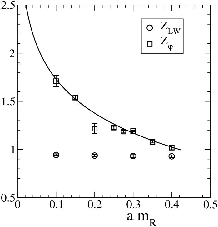
The values of $Z_{\varphi}$ and $Z_{\text{LW}}$ are reported in Fig. 1. As one can check, the two $Z$’s follow completely different trends and the discrepancy becomes larger and larger when approaching the continuum limit, precisely the same behavior observed in Refs.[11, 12, 13]. We also fitted the values for $Z_{\varphi}$ to the form ($\Lambda=\pi/a$)

$$Z_{\varphi}=B\,\ln{(\Lambda/m_{R})}\,.$$ (12)

Notice that the lattice data are completely consistent with the prediction $Z_{\varphi}\sim\ln\Lambda$ of Refs.[4, 7, 5, 6].

Of course, one might object that the discrepancy between lattice data and the perturbative $Z_{\rm LW}$ depends on restricting, for each given $m_{\rm input}$, to the central values of $\kappa$ in the Lüscher-Weisz table. As a matter of fact, there is a theoretical uncertainty in $\kappa$, for each given $m_{\rm input}$, that might be taken into account when comparing with the perturbative $Z_{\rm LW}$’s. For instance, for $m_{\rm input}=0.3$, where the $\kappa$-range predicted in Ref. [21] is $0.0754(2)$, one might also compute $\chi_{\rm latt}$ for $\kappa=0.0756$ (obtaining a value $\chi_{\rm latt}\sim 60$) and for $\kappa=0.0752$ (obtaining a value $\chi_{\rm latt}\sim 130$). As a consequence, for $m_{\rm input}=0.3$, one might also conclude that $Z_{\varphi}$, as defined in Eq.(10), lies in the range $0.8-1.7$, consistently with the prediction of Ref. [21] $Z_{\rm LW}=0.932(13)$.

Adopting this point of view does not represent, however, a solution of the problem. In fact, by inspection of Fig. 1, one can see that the range of $\kappa$-values for which $Z_{\varphi}$, as defined in Eq.(10), is still consistent with the perturbative $Z_{\rm LW}$ becomes smaller and smaller when approaching the continuum limit. As a matter of fact, this range vanishes for $m_{\rm input}\leq 0.08$. This can easily be checked noticing that for $m_{\rm input}=0.08$ Ref. [21] predicts $\kappa=0.07481(8)$, i.e. smaller than $0.0749$. Therefore, by inspection of our Table 2, the lattice susceptibility will be definitely larger than its value for $\kappa=0.0749$, $\chi_{\rm latt}\sim 1100$, so that using Eq.(10), one gets the lower bound $Z_{\varphi}>1.05$. This cannot be reconciled with the perturbative prediction, for $m_{\rm input}=0.08$, $Z_{\rm LW}=0.947(10)$.

In our opinion, one should not ignore this discrepancy, for instance by attempting to further enlarge the error bars of the perturbative predictions so as to reach a marginal consistency with the lattice data. In fact, in this way no meaningful test of perturbation theory will ever be possible. This is in contrast with the situation for the symmetric phase where lattice data and theoretical predictions based on the central values of $\kappa$, as given in Table 3 of Ref. [22], agree to good accuracy, see Refs. [11, 12, 13]. As an additional check, we have computed the zero-momentum susceptibility for the central value $\kappa=0.0741$ that corresponds to $m_{\text{input}}=0.2$. From our result on a $32^{4}$ lattice $\chi_{\text{latt}}=161.94\pm 0.67$, using again Eq. (10), we obtain $Z_{\varphi}=0.960\pm 0.004$ in good agreement with the corresponding Lüscher-Weisz prediction $Z_{\text{LW}}=0.975\pm 0.010$. This is also consistent with the picture of Refs.[4, 5, 6] where the deviations from perturbation theory are only due to the presence of the scalar condensate.

3 Further lattice determination of $Z_{\varphi}$

There is, however, a method to analyze the lattice data where the theoretical uncertainty in the $\kappa-m_{R}$ correlation can be eliminated. In fact, one can perform a fit of the lattice data with the functional form expected in the standard perturbative approach or with the functional form expected in the alternative scenario of Refs.[4, 5, 6]. If this is done, the lattice data confirm a logarithmically divergent $Z_{\varphi}$ in agreement with the previous indications from Fig. 1.

To this end, let us observe that, both in perturbation theory and according to Refs. [4, 5, 6], the bare squared field expectation value $v^{2}_{B}$ is predicted to diverge in units of the physical Higgs boson mass as

$$\frac{v^{2}_{B}}{m^{2}_{R}}\sim\ln{(\Lambda/m_{R})}\,.$$ (13)

Therefore, in the perturbative approach, where the zero-momentum susceptibility is predicted to scale uniformly with the inverse squared Higgs mass, i.e. $\chi_{2}(0)m^{2}_{R}\sim 1$, one expects (PT=Perturbation Theory)

$$\left[v^{2}_{B}\chi_{2}(0)\right]_{\text{PT}}\sim\ln{(\Lambda/m_{R})}\,.$$ (14)

On the other hand, in the approach of Refs. [4, 5, 6] one predicts $Z_{\varphi}=\chi_{2}(0)m^{2}_{R}\sim\ln{(\Lambda/m_{R})}$ so that, in this case, one would rather expect (CS=Consoli-Stevenson)

$$\left[v^{2}_{B}\chi_{2}(0)\right]_{\text{CS}}\sim\ln^{2}{(\Lambda/m_{R})}\,.$$ (15)

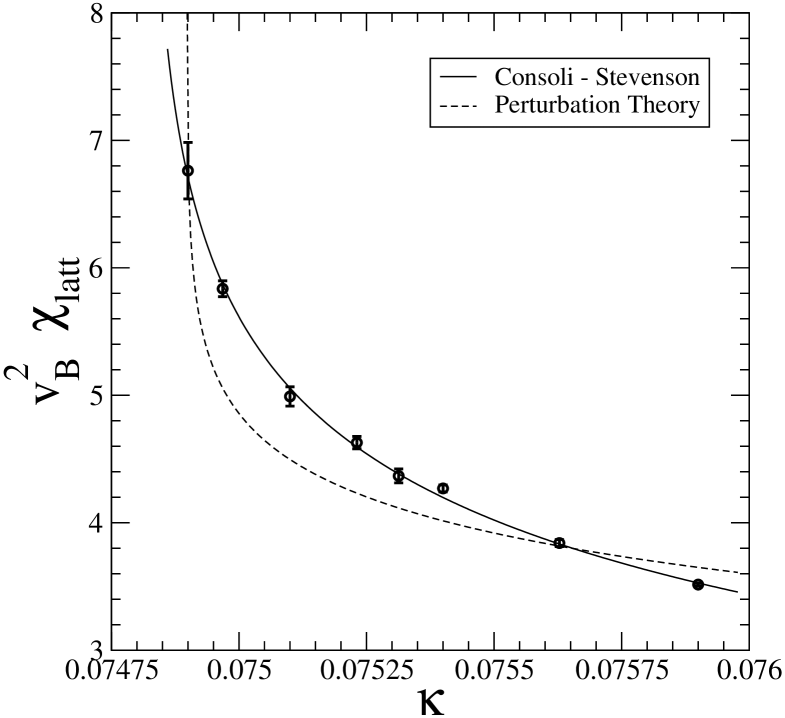
The two predictions in Eq.(14) and in Eq.(15) are free of theoretical uncertainties due to the $\kappa-m_{R}$ correlation and can be directly compared with the lattice data for the product $v^{2}_{B}\chi_{2}(0)$ reported in our Table 3. These data can be fitted to the 3-parameter form

$$\alpha|\ln(\kappa-\kappa_{c})|^{\gamma}$$ (16)

where $\alpha$ is a normalization constant and we shall set the exponent $\gamma=1$, according to Eq.(14), or $\gamma=2$ according to Eq.(15).

Now, fixing $\gamma=1$ one obtains the totally unacceptable value chi-square$\simeq 496$ for 6 degrees of freedom (see Fig. 2). On the other hand, fixing $\gamma=2$, one obtains a good fit of the lattice data (chi-square$\simeq 9$ for 6 degrees of freedom) with a rather precise determination of the critical point from the broken-symmetry phase $\kappa_{c}=0.074818(11)$ consistently with the estimate $\kappa_{c}=0.074834(15)$ from the symmetric phase [23]. This conclusion is also confirmed by the results of the full 3-parameter fit, $\gamma=2.20^{+0.24}_{-0.21}$ and $\kappa_{c}=0.07478(6)$ with a chi-square of 6.4 for 5 degrees of freedom. Therefore, between the two alternatives Eq.(14) and Eq.(15), the lattice data prefer unambiguously the theoretical scenario of Refs. [4, 5, 6].

Before concluding, a brief comment about the Lüscher-Weisz prediction for the product $v^{2}_{B}\chi_{2}(0)$. This is based on the relation

$$\left[v^{2}_{B}\chi_{2}(0)\right]_{\text{LW}}=\frac{3Z_{R}^{2}}{g_{R}}$$ (17)

where $Z_{R}$ and $g_{R}$ are given in Table 3 of Ref. [21] as functions of the mass parameter $m_{R}$.

Therefore, a comparison of Eq.(17) with the lattice data reported in our Table 3 re-introduces unavoidably the uncertainties associated with the $\kappa-m_{R}$ correlation. For instance, for $\kappa=0.0759$ the prediction of Ref. [21] would be $\left[v^{2}_{B}\chi_{2}(0)\right]_{\text{LW}}=4.16$ to be compared with the value $3.5154(122)$ in our Table 3. On the other hand, if one takes into account that the relevant values of $Z_{R}$ and $g_{R}$ in Eq.(17) are actually defined for the mass value $m_{R}=0.4$, for which the entire range is $\kappa=0.0759(2)$, one might also conclude that the theoretical prediction lies in the range $3.76\leq\left[v^{2}_{B}\chi_{2}(0)\right]_{\text{LW}}\leq 4.63$ that, with a short-hand notation, can be expressed as $\left[v^{2}_{B}\chi_{2}(0)\right]_{\text{LW}}=4.20\pm 0.43$.

Notice, however, that the difference between the prediction $4.20\pm 0.43$ and the lattice value $3.5154(122)$ should not be considered a modest $1.6\sigma$ discrepancy. In fact the interval $3.76-4.63$ represents the entire theoretical range allowed by the numerical solution of the renormalization-group equations. At the same time, we observe that the agreement does not seem to improve approaching the continuum limit. For instance, for $m_{R}=0.2$, where the range is $\kappa=0.0751(1)$, Ref. [21] predicts $5.42\leq\left[v^{2}_{B}\chi_{2}(0)\right]_{\text{LW}}\leq 6.31$ to be compared with the lattice value $4.9907(755)$ in our Table 3. This situation might be reminiscent of the discrepancy in the value of $Z_{R}$, pointed out by Jansen et al.  [17], that was not improving when approaching the continuum limit.

4 Summary and outlook

In this paper we have reported the results of a lattice simulation dedicated to check the first numerical indications  [11, 12, 13] for a logarithmically divergent rescaling of the scalar condensate. Two different methods, see Fig. 1 and Fig. 2, support the same behavior $Z_{\varphi}\sim\ln\Lambda$ predicted in Refs. [4, 5, 6] from the analysis of the effective potential.

As anticipated in the Introduction, within this scenario there is one substantial phenomenological implication that concerns the relative scaling of the physical Higgs mass $m_{H}$ and of the physical $v_{R}$ for which $V^{\prime\prime}_{\text{eff}}(v_{R})=m^{2}_{H}$. Namely, once $v^{2}_{R}$ is computed from the bare $v^{2}_{B}$ through Eq.(3) with a value $Z=Z_{\varphi}\sim B\ln\Lambda$, so that

$$v^{2}_{R}\sim v^{2}_{B}~{}\frac{1}{B\ln\Lambda}$$ (18)

this $v^{2}_{R}$ will scale uniformly with

$$m^{2}_{H}\sim v^{2}_{B}~{}\frac{A}{\ln\Lambda}$$ (19)

(where we have set $g_{R}\sim\frac{A}{\ln\Lambda}$).

Therefore, if $v_{R}$ is identified with a physical scale (e.g. $v_{R}\sim 246$ GeV), there are no upper bounds on $m_{H}$ from ‘triviality’ since

$$C=\frac{m_{H}}{v_{R}}\sim\sqrt{AB}$$ (20)

is a cutoff-independent quantity [24]. The numerical value of $C$, however, could depend on the direction chosen to approach the critical line in the more general two-parameter $(\kappa,\bar{\lambda})$ form  [21] of $\Phi^{4}$ theory. Therefore, a new set of lattice simulations is needed to compute the zero-momentum susceptibility $\chi_{\rm latt}$ outside of the Ising limit $\bar{\lambda}=1$.

ACKNOWLEDGEMENTS

We thank P. M. Stevenson for many useful discussions and collaboration.

References

- [1] R. Fernandez, J. Fröhlich, and A. D. Sokal, Random Walks, Critical Phenomena, and Triviality in Quantum Field Theory. Springer-Verlag, Berlin, 1992.
- [2] C. B. Lang, Computer stochastics in scalar quantum field theory, in proceedings of NATO Advanced Study Institute on Stochastic Analysis and Applications in Physics, Funchal, Madeira, 6-19 Aug 1993, hep-lat/9312004.
- [3] R. Kenna, Finite size scaling for O(N) theory at the upper critical dimension, hep-lat/0405023.
- [4] M. Consoli and P. M. Stevenson, The non trivial effective potential of the ’trivial’ theory: a lattice test, Z. Phys. C63 (1994) 427–436, [http://arXiv.org/abs/hep-ph/9310338].
- [5] M. Consoli and P. M. Stevenson, Model-dependent field renormalization and triviality in theory, Phys. Lett. B391 (1997) 144–149.
- [6] M. Consoli and P. M. Stevenson, Physical mechanisms generating spontaneous symmetry breaking and a hierarchy of scales, Int. J. Mod. Phys. A15 (2000) 133, [http://arXiv.org/abs/hep-ph/9905427].
- [7] A. Agodi, G. Andronico, and M. Consoli, Lattice effective potential giving spontaneous symmetry breaking and the role of the Higgs mass, Z. Phys. C66 (1995) 439–452, [hep-lat/9410001].
- [8] P. M. Stevenson, B. Alles, and R. Tarrach, O(N) symmetric theory: the Gaussian effective potential approach, Phys. Rev. D35 (1987) 2407.
- [9] U. Ritschel, I. Stancu, and P. M. Stevenson, Unconventional large N limit of the Gaussian effective potential and the phase transition in theory, Z. Phys. C54 (1992) 627–634.
- [10] U. Ritschel, NonGaussian corrections to Higgs mass in autonomous in (3+1)-dimensions, Z. Phys. C63 (1994) 345–350, [hep-ph/9210206].
- [11] P. Cea, M. Consoli, and L. Cosmai, First lattice evidence for a non-trivial renormalization of the Higgs condensate, Mod. Phys. Lett. A13 (1998) 2361–2368, [http://arXiv.org/abs/hep-lat/9805005].
- [12] P. Cea, M. Consoli, L. Cosmai, and P. M. Stevenson, Further lattice evidence for a large re-scaling of the Higgs condensate, Mod. Phys. Lett. A14 (1999) 1673–1688, [http://arXiv.org/abs/hep-lat/9902020].
- [13] P. Cea, M. Consoli, and L. Cosmai, Large rescaling of the Higgs condensate: Theoretical motivations and lattice results, Nucl. Phys. Proc. Suppl. 83 (2000) 658–660, [hep-lat/9909055].
- [14] M. Lüscher, A portable high quality random number generator for lattice field theory simulations, Comput. Phys. Commun. 79 (1994) 100–110, [hep-lat/9309020].
- [15] F. James, Ranlux: A fortran implementation of the high quality pseudorandom number generator of Lüscher, Comp. Phys. Commun. 79 (1994) 111–114.
- [16] L. N. Shchur and P. Butera, The ranlux generator: Resonances in a random walk test, Int. J. Mod. Phys. C9 (1998) 607–624, [hep-lat/9805017].
- [17] K. Jansen, T. Trappenberg, I. Montvay, G. Munster, and U. Wolff, Broken phase of the four-dimensional Ising model in a finite volume, Nucl. Phys. B322 (1989) 698.
- [18] I. Montvay and P. Weisz, Numerical study of finite volume effects in the four- dimensional ising model, Nucl. Phys. B290 (1987) 327.
- [19] R. H. Swendsen and J.-S. Wang, Nonuniversal critical dynamics in Monte Carlo simulations, Phys. Rev. Lett. 58 (1987) 86–88.
- [20] U. Wolff, Collective Monte Carlo updating for spin systems, Phys. Rev. Lett. 62 (1989) 361.
- [21] M. Lüscher and P. Weisz, Scaling laws and triviality bounds in the lattice theory. 2. One component model in the phase with spontaneous symmetry breaking, Nucl. Phys. B295 (1988) 65.
- [22] M. Lüscher and P. Weisz, Scaling laws and trivality bounds in the lattice theory. 1. One component model in the symmetric phase, Nucl. Phys. B290 (1987) 25.
- [23] D. S. Gaunt, M. F. Sykes, and S. McKenzie J. Phys. A12 (1979) 871.
- [24] P. Cea, M. Consoli, and L. Cosmai, Indications on the Higgs boson mass from lattice simulations, Nucl. Phys. Proc. Suppl. 129 (2004) 780–782, [hep-lat/0309050].