Mobility edge in lattice QCD

Abstract

We determine the location $\lambda_{c}$ of the mobility edge in the spectrum of the hermitian Wilson operator on quenched ensembles. We confirm a theoretical picture of localization proposed for the Aoki phase diagram. When $\lambda_{c}>0$ we also determine some key properties of the localized eigenmodes with eigenvalues $|\lambda|<\lambda_{c}$. Our results lead to simple tests for the validity of simulations with overlap and domain-wall fermions.

Localization of electronic wave functions is a familiar phenomenon in disordered systems DJT . Recently we conjectured lcl that a similar phenomenon takes place in lattice QCD with Wilson fermions: In an ensemble of gauge configurations, the low-lying eigenmodes of the hermitian Wilson operator can be localized, up to some mobility edge above which they become extended. This observation has two important applications. First, it helps resolve a paradox in the quenched theory with negative bare mass $m_{0}$, where simulations with two valence quarks have discovered a condensate that breaks the isospin symmetry in regions without Goldstone bosons scri . Second, there are important implications for large-scale simulations of QCD with domain-wall dwf and overlap overlap fermions. Both of these formulations are based on Wilson fermions with negative $m_{0}$. Quenched as well as unquenched calculations with these fermions will thus be sensitive to the spectrum of the Wilson operator. It turns out that an understanding of the localization properties is important for ensuring chirality and locality.

In two-flavor QCD with Wilson fermions, part of the “supercritical” region ($-8<m_{0}<0$) is the so-called Aoki phase aoki , where a pion condensate $\langle\pi_{3}\rangle$ breaks both parity and isospin symmetry. Inside the Aoki phase one pion is massive, whereas the other two pions are Goldstone bosons. Outside the Aoki phase (e.g., for weak coupling, away from the critical values $m_{0}=0,$ $-2,$ $\ldots$) all pions are massive.

It is this supercritical massive phase that presents the conundrum in the quenched theory. The word “quenched” here can refer to any ensemble of gauge configurations generated without the Wilson-fermion determinant, whether a pure gauge ensemble or an ensemble with dynamical fermions of some other type, such as domain-wall fermions . Both the massless and the massive supercritical phases support a non-zero density of near-zero eigenmodes, and hence a condensate through the Banks–Casher relation $\left\langle\pi_{3}\right\rangle=2\pi\rho(0)$ BC , where $\rho(\lambda)$ is the spectral density of the hermitian Wilson operator $H_{W}$. Why are there no Goldstone bosons? In Ref. lcl, we proposed a detailed physical picture which resolves this puzzle. A key observation (first made in Ref. ms, ) is that, in a quenched system, localization provides an alternative to the Goldstone theorem. In this Letter we present numerical evidence supporting and illustrating this picture. The implications for domain-wall and overlap fermions are thus made more concrete.

In order to develop this physical picture, we probe our quenched ensemble with the two-flavor fermion action

$$S_{F} = \bar{\psi}(D-(\lambda+i\tau_{3}m_{1})\gamma_{5})\psi$$ (1)

$$= \bar{\psi}(H_{W}-(\lambda+i\tau_{3}m_{1}))\psi^{\prime},$$

where $\psi^{\prime}=\gamma_{5}\psi$, and $\tau_{k}$ are Pauli matrices acting in flavor space. $H_{W}=D\gamma_{5}$ is hermitian. Explicitly,

$$D=\left(\begin{array}[]{cc}W+m_{0}&-C\\ C^{\dagger}&W+m_{0}\end{array}\right),$$ (2)

where $C_{xy}={1\over 2}\sum_{\mu=1}^{4}\left(\delta_{x+\hat{\mu},y}U_{x\mu}-\delta_{x-\hat{\mu},y}U^{\dagger}_{y\mu}\right)\sigma_{\mu}$ and $W_{xy}=4\delta_{xy}-{1\over 2}\sum_{\mu=1}^{4}\left(\delta_{x+\hat{\mu},y}U_{x\mu}+\delta_{x-\hat{\mu},y}U^{\dagger}_{y\mu}\right)$. Each entry is a $2\times 2$ matrix, with $\sigma_{\mu}=(\vec{\sigma},i)$, and $\sigma_{k}$ three Pauli spin matrices. The link variables $U_{x\mu}\in SU(3)$ constitute the random field in which the fermions move. The parameter $\lambda$ will allow us to study the spectral density $\rho(\lambda)$ of $H_{W}$ via a condensate. $m_{1}$ is a “twisted mass” which breaks isospin aoki ; tm , and acts as an external magnetic field for the condensate of interest. Neither $\lambda$ nor $m_{1}$ appears in the Boltzmann weight of the ensemble.

For any $\lambda$ and $m_{1}$ one derives the Ward identity

$$\sum_{\mu}\partial^{*}_{\mu}\left\langle J^{+}_{\mu}(x)\,\pi^{-}(y)\right\rangle+2m_{1}\left\langle\pi^{+}(x)\,\pi^{-}(y)\right\rangle\!=\!\delta_{xy}\left\langle\pi_{3}(y)\right\rangle.$$ (3)

Here $\partial^{*}_{\mu}f(x)=f(x)-f(x-\hat{\mu})$ and $J^{+}_{\mu}(x)$ is the flavor-changing vector current , and $\pi^{\pm}=i\bar{\psi}\gamma_{5}\tau_{\pm}\psi$ and $\pi_{3}=i\bar{\psi}\gamma_{5}\tau_{3}\psi$, with $\tau_{\pm}=(\tau_{1}\pm i\tau_{2})/2$. Introducing the Green function $G=(H_{W}-\lambda-im_{1})^{-1}$ one has

$$\left\langle\pi_{3}\right\rangle=(2/V_{4})\,{\rm Im\,}{\rm tr}\,\left\langle G\right\rangle,$$ (4)

where $V_{4}$ is the four-volume. This implies a generalized Banks–Casher relation

$$\lim_{m_{1}\to 0}\left\langle\pi_{3}\right\rangle=2\pi\rho(\lambda).$$ (5)

Thus the spectral density $\rho(\lambda)$ is an order parameter for flavor symmetry breaking in the quenched theory with fermion action (1). The easiest way to calculate $\rho(\lambda)$ is in fact through Eqs. (4) and (5).

The two-point function $\Gamma(x,y;\lambda)=\left\langle\pi^{+}(x)\,\pi^{-}(y)\right\rangle$ represents correlations of the eigenmode densities of $H_{W}$. This is readily seen from its spectral decomposition,

$$\Gamma(x,y;\lambda) = \left\langle\sum_{kn}\Psi_{n}^{\dagger}(x)\Psi_{k}(x){1\over\lambda_{k}-\lambda+im_{1}}\right.$$ (6)

$$\left.\times\Psi_{k}^{\dagger}(y)\Psi_{n}(y){1\over\lambda_{n}-\lambda-im_{1}}\right\rangle,$$

where $\Psi_{n}$ is the eigenmode of $H_{W}$ with eigenvalue $\lambda_{n}$. We calculate it at zero three-momentum, $\Gamma(t;\lambda)=(\pi V_{3})^{-1}\sum_{\vec{x}\vec{y}}\Gamma(0,\vec{x},t,\vec{y};\lambda)$, where $V_{3}$ is the spatial volume. The mobility edge $\lambda_{c}$ is determined as the value of $\lambda$ where these correlations become long-ranged as $m_{1}\to 0$, that is, when the large-$t$ behavior of $\Gamma(t;\lambda)$ changes from exponential ($0\leq|\lambda|<\lambda_{c}$) to power law ($|\lambda|>\lambda_{c}$) in this limit. Above $\lambda_{c}$ one has extended modes, and the long-range density–density correlations play the role of Goldstone bosons for flavor symmetry breaking. Below $\lambda_{c}$ there are no long-range correlations, and no massless pole in $\left\langle J^{+}_{\mu}(x)\,\pi^{-}(y)\right\rangle$. How, then, can the Ward identity (3) be satisfied in the limit $m_{1}\to 0$? The answer is that, when $\rho(\lambda)$ arises from exponentially localized modes, the quenched two-point function $\Gamma(x,y;\lambda)$ diverges as $1/m_{1}$ in this limit ms ; lcl . In fact ,

$$\Gamma(x,y;\lambda)\!\!\! = \!\!\!{1\over m_{1}}\left\langle\sum_{n}|\Psi_{n}(x)|^{2}|\Psi_{n}(y)|^{2}{m_{1}\over(\lambda_{n}-\lambda)^{2}+m_{1}^{2}}\right\rangle$$ (7)

$$\quad+O(1).$$

As $m_{1}\to 0$, the expectation value in Eq. (7) is non-zero if and only if $\rho(\lambda)\neq 0$. It thus provides a mechanism for saturating the Ward identity without Goldstone bosons.

If the mobility edge is at $\lambda=0$, Goldstone bosons dominate the correlation function; hence we may take $\lambda_{c}=0$ to be the definition of the Aoki phase.

We have determined the value of $\lambda_{c}$ at several locations in the $(\beta,m_{0})$ plane. For each value of $\beta$ we generated an ensemble of 120 quenched configurations using the standard plaquette action. The four-volume was $16^{4}$, with periodic boundary conditions for all fields. Our measurements were mostly done at $m_{0}=-1.5$ [hopping parameter $\kappa=(8+2m_{0})^{-1}=0.2$], which is roughly the value used in domain-wall and overlap simulations. We measured $\Gamma(t;\lambda)$ using random sources on time slices 0 and $t$. We extracted a mass $M=M(\lambda,m_{1})$ from $\Gamma(t;\lambda)$ at $m_{1}$ values between 0.01 and 0.07, and extrapolated to $m_{1}=0$ by fitting to $M^{2}=\mu^{2}(\lambda)+\alpha(\lambda)\,m_{1}$ . The results for $\beta=5.85$ are shown in the second column of Table 1. One sees that $\mu^{2}$ starts falling rapidly above $\lambda=0.1$.

Table 1: Exponential falloff rate of the density–density correlator $\Gamma(t;\lambda)$ at $\beta=5.85$, $m_{0}=-1.5$, for $m_{1}\to 0$. Errors are statistical only. $\mu$ is the extrapolation of masses determined at $m_{1}\neq 0$, while $\tilde{\mu}$ is extracted by extrapolation of $m_{1}\Gamma(t;\lambda)$ to $m_{1}=0$.

. $\lambda$ $\mu^{2}$ $\tilde{\mu}^{2}$ $0.0$ $2.42(6)$ 1.9–2.3 $0.1$ $1.99(8)$ 1.3–1.9 $0.2$ $1.18(5)$ 0.9–1.1 $0.3$ $0.21(3)$ 0.4–0.5 $0.4$ $-0.04(2)$ 0.12 $0.5$ $-0.04(2)$ 0.05 $0.6$ $-0.05(2)$ 0.01

By definition $\mu^{2}(\lambda)$ drops to zero at the mobility edge $\lambda_{c}$. We determine $\lambda_{c}$ by linear extrapolation from the last two points with positive $\mu^{2}$. Our results are compiled in Table 2. Consider first the $m_{0}=-1.5$ results. For reference, we include the free-theory limit ($\beta=\infty$) lcl , where $\lambda_{c}$ coincides with the gap of the free $H_{W}$. At $\beta=6.0$, $\lambda_{c}$ is still close to its free-field value. The curve $\lambda_{c}(\beta)$ steepens before reaching zero somewhere between $\beta=5.6$ and $\beta=5.5$, where we enter the Aoki phase.

Table 2: Mobility edge $\lambda_{c}(\beta,m_{0})$ and (when $\lambda_{c}>0$) interpolated spectral density $\rho(\lambda_{c})$. Where no error is shown, the (statistical) error is less than one in the last digit.

$\beta$	$m_{0}$	$\lambda_{c}$	$\rho(\lambda_{c})$
$\infty$	$-1.5$	$0.5$
$6.0$	$-1.5$	$0.41$	0.14
$5.85$	$-1.5$	$0.32$	0.08
$5.7$	$-1.5$	$0.25$	0.07
$5.6$	$-1.5$	$0.14(2)$	0.05
$5.5$	$-1.5$	$0.0$	–
$5.4$	$-1.5$	$0.0$	–
$5.7$	$-2.0$	$0.21$	0.14
$5.7$	$-2.4$	$0.03(2)$	0.06

Table 2 also shows results at two other $m_{0}$ values for $\beta=5.7$. The $m_{0}=-2.4$ result suggests that one is near the boundary of the Aoki phase . We find only a small change between $m_{0}=-2.0$ and $m_{0}=-1.5$, consistent with the finding of Ref. scri, that the spectral properties of $H_{W}$ vary slowly over this range. This is why we have explored mainly the $\beta$-dependence at fixed $m_{0}=-1.5$.

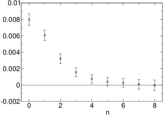
Figure 1: Coefficient of the $1/m_{1}$-divergence in $\tilde{\Gamma}(\omega_{n};\lambda)$ for $\beta=5.7$, $m_{0}=-1.5$, $\lambda=0.0$.

In order to account lcl for the absence of a massless pole in Eq. (3), the $1/m_{1}$-divergence in $\Gamma(x,y;\lambda)$ must persist for a range of momenta $p$, and its coefficient should depend smoothly on $p$. To confirm this, we calculated the Fourier transform $\tilde{\Gamma}(\omega_{n};\lambda)=\sum_{t}\cos(\omega_{n}t)\Gamma(t;\lambda)$, where $\omega_{n}=2\pi n/16$, and extrapolated $m_{1}\tilde{\Gamma}(\omega_{n};\lambda)$ linearly to $m_{1}=0$ . Results are shown in Fig. 1 for $\lambda=0.0$ at $(\beta,m_{0})=(5.7,-1.5)$. The $\omega$-dependence of the $1/m_{1}$-divergence is indeed smooth. For comparison, we repeated the calculation for $\lambda=0.5$, which is above $\lambda_{c}$. The extrapolation of $m_{1}\tilde{\Gamma}(0;\lambda)$ to $m_{1}=0$ is straightforward, as it must be since this gives $\rho(\lambda)$ according to Eqs. (3) and (5). Doing the same with $\tilde{\Gamma}(\omega_{n}\neq 0;\lambda)$, however, leads to a huge $\chi^{2}$. This confirms the qualitative difference between $|\lambda|<\lambda_{c}$ and $|\lambda|>\lambda_{c}$.

We present in Table 3 some quantities that further illustrate properties of the localized modes, for the same $(\beta,m_{0})$ as in Table 1. Using them, we can address the question of whether below the mobility edge $\rho(\lambda)$ arises from well-separated, exponentially localized eigenmodes.

Table 3: Spectral properties for $\beta=5.85$, $m_{0}=-1.5$. The mobility edge is at $\lambda_{c}=0.32$, marked by the horizontal line in the table.

$\lambda$	$\rho(\lambda)$	$R$	$l_{s}$	$l_{l}$
$0.0$	0.0011(1)	$17.$	$3.1(4)$	$0.64(1)$
$0.1$	0.0019(1)	$15.$	$3.5(5)$	$0.71(1)$
$0.2$	0.0088(4)	$10.$	$3.7(4)$	$0.92(2)$
$0.3$	0.056(1)	$6.5$	$4.3(3)$	$2.2(2)$
$0.4$	0.168(7)	$4.9$	$4.7(8)$	$-$
$0.5$	0.27(1)	$4.4$	$11.(3)$	$-$
$0.6$	0.39(2)	$4.0$	$7.(1)$	$-$

We define a generalized “participation ratio” ${\cal P}_{n}$ for a single eigenmode via ${\cal P}_{n}^{-1}=\sum_{t}(\sum_{\vec{x}}|\Psi_{n}(\vec{x},t)|^{2})^{2}$ DJT . If $|\Psi_{n}|^{2}$ has support mainly on a four-volume $l_{n}^{4}$, then ${\cal P}_{n}\sim l_{n}$. A spectral decomposition of the quantity ${\cal P}^{-1}(\lambda)=\lim_{m_{1}\to 0}m_{1}\Gamma(t=0;\lambda)$ shows that it is equal to $\rho(\lambda)$ times an average of ${\cal P}_{n}^{-1}$ over eigenmodes with eigenvalue $\lambda_{n}=\lambda$. Thus, if we define the “support length” $l_{s}=\rho(\lambda){\cal P}(\lambda)$, we see that $1/l_{s}$ is an average of $1/l_{n}$. The fourth column of Table 3 gives this $l_{s}$, a measure of the linear size of the support of the eigenmodes.

We may now compare $l_{s}$ to the distance between eigenmodes. We have a measure of the latter from the values of $m_{1}$ that we used in measuring $\rho(\lambda)$. Spectral sums as in Eq. (7) show that $m_{1}$ is the resolution with which we detect eigenmodes near $\lambda$. For $m_{1}\simeq 0.01$, the number of modes we detect for a typical gauge configuration is thus $N\simeq 0.01V_{4}\rho(\lambda)$, and so $R(\lambda)=(0.01\,\rho(\lambda))^{-1/4}$ is a measure of the average distance between modes. If $l_{s}\ll R$ the modes are isolated, and correlation functions reflect properties of individual localized modes, with no interference. Table 3 shows this to be the case well below the mobility edge.

The density of an exponentially localized mode has the asymptotic behavior

$$|\Psi(x)|^{2}\sim c\,\exp(-|x-x_{0}|/l_{l}),$$ (8)

which defines $l_{l}$, the localization length. When the modes are isolated, the decay rate (extrapolated to $m_{1}=0$) of $\Gamma(t;\lambda)$ reflects the localization length of the individual modes. We thus define an average localization length through $l_{l}=1/\mu$ (Table 3, last column; compare Table 1, 2nd column). Well below the mobility edge $l_{l}$ turns out to be much smaller than $l_{s}$. In fact, for $\beta\geq 5.85$, we find that $l_{l}<1$ and $l_{s}>3$. This is good news for domain-wall and overlap simulations (see below).

Equation (8) represents an exponential envelope that we expect to multiply oscillations in $|\Psi_{n}|^{2}$. These fluctuations, often large, survive the extrapolation of the correlation function $\Gamma(t;\lambda)$ itself to $m_{1}=0$. As a result, if we extract a mass $\tilde{\mu}$ from $\lim_{m_{1}\to 0}m_{1}\Gamma(t;\lambda)$, the result varies with the details of the fit. We present rough values of $\tilde{\mu}$ in the last column of Table 1. In the absence of a model for the fluctuations, $\tilde{\mu}$ is only a qualitative measure, and hence we do not quote an error. $\tilde{\mu}$ follows the trends shown by $\mu$.

Taking all our results together, we have compelling evidence for exponential localization well below the mobility edge. Here the modes are isolated in the sense of $l_{s}\ll R$ (for $m_{1}\simeq 0.01$), and $l_{l}=1/\mu$ provides an accurate estimate of the average localization length. For $\lambda\gtrsim\lambda_{c}$ interference effects destroy this connection. Upon comparing our data for all values of $(\beta,m_{0})$ shown in Table 2, we find that we can characterize the mobility edge itself as follows: (1) $\rho(\lambda)\approx 0.05$–$0.15$ near $\lambda_{c}$; (2) $l_{l}\gtrsim 1$ signals the proximity of $\lambda_{c}$; (3) $l_{s}\simeq R\simeq 5$ at $\lambda_{c}$ future .

Finally, we revisit the implications of our results for domain-wall and overlap fermions. These two closely related descendants of Wilson fermions employ a super-critical Wilson operator as a key element in their construction. Both are expected to be local, and they both have a (modified) chiral symmetry Luscher at non-zero lattice spacing. The question is to what extent these expectations are fulfilled in actual lattice QCD simulations employing these fermions. In Ref. lcl, we argued that locality and chirality will coexist in these formulations if and only if the following holds: On a given ensemble of configurations, the mobility edge of the underlying Wilson operator must be well above zero. It does not matter whether the ensemble is quenched or is generated with dynamical domain-wall or overlap fermions. We will not repeat the whole argument lcl here but rather focus on assessing the implications of our numerical results.

Domain-wall fermions employ an auxiliary, discrete, and (in practice) finite fifth dimension with spacing $a_{5}$ and $N_{s}$ sites. Finiteness of the fifth dimension ensures locality but leads to “residual” violations of chiral symmetry. A common measure of these violations, denoted as $m_{\text{res}}$, may be thought of as an additive correction to the quark mass. It is determined from a ratio of pseudoscalar correlation functions at zero spatial momentum and time separation $t$. In Ref. lcl, it was argued that

$$m_{\text{res}}\sim c_{1}\exp\left(-\tilde{\lambda}_{c}N_{s}\right)+c_{2}\exp\left[-t\left(\tilde{l}_{l}(0)^{-1}-m_{\pi}\right)\right],$$ (9)

where the two terms arise from extended and localized modes, respectively. $m_{\pi}$ is the pion mass in the simulation. The mobility edge $\tilde{\lambda}_{c}$ and the localization length $\tilde{l}_{l}(\lambda=0)$ refer to a “hamiltonian” $\tilde{H}$ obtained from the transfer matrix in the fifth dimension, which depends on $a_{5}$. Thus $m_{\text{res}}$ reflects the spectral properties of $\tilde{H}$. We recover $H_{W}$ from $\tilde{H}$ in the limit $a_{5}\to 0$. Moreover, it can be proved that $\tilde{H}\Psi=0$ if and only if $H_{W}\Psi=0$, i.e. the zero modes of $\tilde{H}$ remain unchanged as $a_{5}$ is varied. This implies that $\tilde{l}_{l}(0)=l_{l}(0)$. For quenched simulations at $\beta\gtrsim 5.85$ we thus find that $\tilde{l}_{l}(0)=l_{l}(0)\simeq 0.6$. The last term in Eq. (9) therefore vanishes rapidly with $t$. This agrees with previous findings mres that $m_{\text{res}}$ is fairly $t$-independent once $t$ is large enough. Similarly, $\tilde{\lambda}_{c}=0$ if and only if $\lambda_{c}=0$. Since good chiral symmetry requires $m_{\text{res}}$ to be small, it follows that simulations must be performed well outside the Aoki phase of the underlying Wilson operator.

For overlap fermions, chiral symmetry is guaranteed, but not locality. Deteriorating locality may distort physical predictions in an uncontrolled way. Indeed, for large separations one expects $D_{\text{ov}}(x,y)\sim c_{\text{ov}}\exp(-|x-y|/l_{\text{ov}})$. The exponential tail of the overlap may be represented as an unphysical field of mass $1/l_{\text{ov}}$ that mixes with the physical quarks with an amplitude controlled by $c_{\text{ov}}$. The range of the overlap operator, far from being merely a numerical nuisance, is thus a key indicator of the validity of a simulation.

If an admissibility condition is imposed, it can be proved that the range $l_{\text{ov}}$ of the overlap operator is $O(1)$ in lattice units hjl . For realistic ensembles, $l_{\text{ov}}$ depends on the spectral properties of $H_{W}$, and good locality again requires keeping away from the Aoki phase. One anticipates that $l_{\text{ov}}$ is on the order of either $\lambda_{c}^{-1}$ or $l_{l}(0)$, whichever is larger; if it is the latter, $c_{\text{ov}}$ should be related to $\rho(0)$ lcl . The spectral properties studied in this Letter are thus of central importance for understanding the locality properties of the overlap operator.

- (1) See for example D.J. Thouless, Phys. Rep. 13, 93 (1974).
- (2) M. Golterman and Y. Shamir, Phys. Rev. D 68, 074501 (2003); Nucl. Phys. Proc. Suppl. 129, 149 (2004).
- (3) R.G. Edwards, U.M. Heller and R. Narayanan, Nucl. Phys. B522, 285 (1998); B535, 403 (1998); Phys. Rev. D 60, 034502 (1999) .
- (4) D. B. Kaplan, Phys. Lett. B 288, 342 (1992); Y. Shamir, Nucl. Phys. B 406, 90 (1993); V. Furman and Y. Shamir, Nucl. Phys. B 439, 54 (1995).
- (5) H. Neuberger, Phys. Lett. B 417, 141 (1998); 427, 353 (1998); Phys. Rev. D 57, 5417 (1998).
- (6) S. Aoki, Phys. Rev. D 30, 2653 (1984); 33, 2399 (1986); 34, 3170 (1986). See also S. R. Sharpe and R. J. Singleton, Phys. Rev. D 58, 074501 (1998).
- (7) T. Banks and A. Casher, Nucl. Phys. B169, 103 (1980).
- (8) A.J. McKane and M. Stone, Ann. Phys. (NY) 131, 36 (1981).
- (9) R. Frezzotti, P. A. Grassi, S. Sint and P. Weisz, J. High Energy Phys. 0108, 058 (2001).
- (10) A. Ali Khan et al. [CP-PACS Collaboration], Phys. Rev. D 63, 114504 (2001); Y. Aoki et al. [RBRC collaboration], Phys. Rev. D 69, 074504 (2004).
- (11) M. Golterman, Y. Shamir, and B. Svetitsky, in preparation.
- (12) M. Lüscher, Phys. Lett. B 428, 342 (1998).
- (13) P. Hernández, K. Jansen and M. Lüscher, Nucl. Phys. B552, 363 (1999).