BI-TP 2004/14 FTUV-04-0705

CPT-2004/P.031 IFIC/04-29

DESY 04-081 MPP-2004-55

A strategy to study the rôle of the charm quark
in explaining the $\Delta{I}=1/2$ rule

L. Giusti^a, P. Hernández^b, M. Laine^c, P. Weisz^d, H. Wittig^e
a Centre de Physique Théorique, Case 907, CNRS Luminy

F-13288 Marseille Cedex 9, France ^b Dpto. Física Teórica and IFIC, Edificio Institutos Investigación,

Apt. 22085, E-46071 Valencia, Spain ^c Faculty of Physics, University of Bielefeld,

D-33501 Bielefeld, Germany ^d Max-Planck-Institut für Physik, Föhringer Ring 6,

D-80805 Munich, Germany ^e DESY, Theory Group, Notkestrasse 85,

D-22603 Hamburg, Germany
Abstract

We present a strategy designed to separate several possible origins of the well-known enhancement of the $\Delta{I}=1/2$ amplitude in non-leptonic kaon decays. In particular, we seek to unambiguously quantify the rôle of the charm quark mass in the observed enhancement. This is achieved by considering QCD with an unphysically light charm quark, so that the theory possesses an approximate ${\rm SU(4)_{L}\times SU(4)_{R}}$ chiral symmetry. The strategy proceeds by computing the relevant operator matrix elements and monitoring their values as the charm quark mass departs from the SU(4)-symmetric situation. We study the influence of the charm quark mass in Chiral Perturbation Theory. First results from lattice simulations in the SU(4)-symmetric limit are also discussed.

December 2004

1 Introduction

A quantitative understanding of non-leptonic kaon decays, such as $K\to\pi\pi$, has been elusive for many years, and thus the explanation of the famous $\Delta{I}=1/2$ rule or the value of $\epsilon^{\prime}/\epsilon$ has remained a longstanding problem. Early analyses have shown that, in a Standard Model-based explanation, the bulk of the enhancement of the $\Delta{I}=1/2$ amplitude must be due to long-distance contributions generated by the strong interactions [?]. A reliable determination of these effects must inevitably be performed at the non-perturbative level [?,?]. Currently, lattice simulations of QCD are the only known methodology which can achieve this goal with controlled systematic errors. Lattice studies of $K\to\pi\pi$ decays have, however, been hampered by a number of technical difficulties, for instance by the so-called Maiani-Testa No-Go Theorem [?], which states that transition amplitudes of two-body decays cannot simply be obtained from the asymptotic behaviour of Euclidean correlation functions computed in very large volumes. In addition, lattice calculations employing commonly used Wilson fermions need non-perturbative subtractions of power divergences for defining properly renormalised operators which enter the effective weak Hamiltonian [?]. Thus, efforts to investigate the $\Delta{I}=1/2$ rule numerically on the lattice had practically come to a halt during most part of the 1990s.

Recently, it was realised, though, that the Maiani-Testa Theorem does not apply to volumes with linear extensions of a few fm, and a relation between the physical two-body decay rate and the square of the transition matrix element in finite volume could be derived [?] (for subsequent work, see [?]). Furthermore, the advent of fermionic discretisations which preserve chiral symmetry at non-zero lattice spacing (Ginsparg-Wilson fermions) [?,?,?,?,?,?,?,?,?], has alleviated the mixing problem to the extent that the renormalisation patterns of four-fermion operators mediating $\Delta{S}=1$ transitions are like in the continuum [?]. These developments have removed the main obstacles for a lattice treatment of non-leptonic kaon decays, based on first principles. An approximate realisation of Ginsparg-Wilson fermions via the so-called Domain Wall formulation has already been applied to non-leptonic kaon decays with some success [?,?].

The decay of a neutral kaon into a pair of pions in a state with isospin $I$ is described by the transition amplitude

$$T(K^{0}\to\pi\pi\big{|}_{I=\alpha})=iA_{\alpha}{\rm e}^{i\delta_{\alpha}},\qquad\alpha=0,\,2,$$ (1.1)

where $\delta_{\alpha}$ is the scattering phase shift. In this paper we focus on the $\Delta{I}=1/2$ rule, i.e. the empirical observation that the amplitude $|A_{0}|$ is significantly larger than $|A_{2}|$,

$$|A_{0}|/|A_{2}|=22.1.$$ (1.2)

There are several possible sources for an enhancement due to strong interaction effects. These involve physics at the scale of the charm quark, i.e. at around 1 GeV, physics at an intrinsic QCD scale $E_{\rm QCD}\approx 250\,{\rm MeV}$, and effects due to pionic final state interactions at around 100 MeV. It remains unclear, though, whether the enhancement is the result of an accumulation of several effects, each giving a moderate contribution, or whether it is mainly due to a single cause or mechanism.

The possible rôle of the charm quark has been pointed out long ago in ref. [?]: for energy scales $E\ll m_{c}$ the GIM mechanism no longer operates, which gives rise to so-called “penguin operators” that mediate $\Delta{I}=1/2$ transitions. The commonly accepted scenario that the $\Delta{I}=1/2$ rule arises predominantly from long-distance QCD contributions has been supported by several analytical [?,?,?,?,?] and numerical [?,?] studies.

In this paper we describe a general strategy which allows to disentangle contributions from the various sources and quantify them using numerical simulations. The main idea is to keep an active charm and determine the leading low-energy constants (LECs) associated with the CP conserving $\Delta S=1$ weak Hamiltonian of the chiral low-energy effective theory as a function of the charm quark mass. These parameters can be determined by computing suitable correlation functions at small masses and momenta in a lattice simulation and comparing them with the predictions of Chiral Perturbation Theory (ChPT). If the charm is degenerate with the light quarks, $m_{u}=m_{d}=m_{s}=m_{c}$, the theory has an exact $\rm SU(4)_{L}\times SU(4)_{R}$ symmetry in the chiral limit, which is broken explicitly by the weak interactions. In this situation the calculation of the LECs corresponding to $\Delta{I}=1/2$ and 3/2 transitions will expose any QCD contribution to the enhancement at scales around $E_{\rm{QCD}}$. The effect of a heavier charm quark can then be isolated by monitoring the amplitudes as $m_{c}$ departs from the degenerate limit: $m_{c}>m_{u}=m_{d}=m_{s}$. By keeping an active charm quark and employing a lattice formulation which preserves chiral symmetry, power-divergent subtractions of the relevant operators can be avoided, and small quark masses can be simulated without numerical instabilities.

Since simulations with dynamical Ginsparg-Wilson fermions are still prohibitively expensive, it is reasonable to perform initial tests of our proposed strategy in the quenched approximation. It is well known, though, that the quenched theory is afflicted with several problems, whose implications are discussed in detail in the relevant sections below. In order to illustrate our strategy, we present first numerical results for the SU(4)-symmetric case obtained in the quenched approximation for quark masses near $m_{s}/2$. Numerical results for smaller masses and the investigation of the dependence on the charm quark mass are left to future publications.

The outline of the remainder of this paper is as follows: in Sect. 2 we discuss the effective weak interactions with an active charm quark. The lattice-regularised theory, formulated using Ginsparg-Wilson quarks, is described in Sect. 3. The renormalisation group invariant formulation of the effective weak Hamiltonian is addressed in Sect. 4. In Sect. 5 we discuss the effective low-energy description of $\Delta{S}=1$ weak interactions in terms of ChPT in a finite volume. The decoupling of the charm quark for small quark masses, i.e. $m_{c}\;\raisebox{-2.58334pt}{$\stackrel{{\scriptstyle\textstyle{>}}}{{\sim}}$}\;m_{u},m_{d},m_{s}$, is analysed in Sect. 6 using ChPT. Our numerical results are discussed in Sect. 7, and in Sect. 8 we present our conclusions. In several appendices we provide further information on the SU(4) classification of operators, the transformation properties of four-quark operators in the lattice theory, the perturbative renormalisation of four-quark operators using overlap fermions, as well as details of the calculations performed in finite-volume ChPT.

2 The effective weak interactions with an active charm quark

In this section we collect some basic facts and definitions regarding the $\Delta{S}=1$ effective weak interaction, focusing on the less familiar case of an active charm quark. Throughout this paper we work in Euclidean space-time.

2.1 Operator product expansion and global symmetries

The decay of a (neutral or charged) kaon into two pions is induced by charged-current weak interactions, mediated via the exchange of a $W$-boson. It can be described in terms of an effective $V-A$ current-current interaction, i.e.

$$S_{\rm w}={\textstyle\frac{1}{2}}g_{\rm w}^{2}\sum_{q=u,c,t}(V_{qs})^{*}V_{qd}\int{\rm d}^{4}x\,{\rm d}^{4}y\,(\overline{s}\gamma_{\mu}P_{-}q)(x)\,D_{\mu\nu}(x-y)\,(\overline{q}\gamma_{\nu}P_{-}d)(y),$$ (2.3)

where $g_{\rm{w}}^{2}=4\sqrt{2}G_{\rm F}M_{W}^{2}$, $V_{qs},\,V_{qd}$ denote elements of the CKM matrix, $P_{-}=\frac{1}{2}(1-\gamma_{5})$, and $D_{\mu\nu}$ is the propagator of the $W$-boson. Contributions from the top-quark are suppressed by three orders of magnitude relative to those from the up-quark and can thus be safely neglected. At this level of accuracy one has $(V_{us})^{*}V_{ud}=-(V_{cs})^{*}V_{cd}$, so that

$$S_{\rm w} = {\textstyle\frac{1}{2}}g^{2}_{\rm{w}}(V_{us})^{*}V_{ud}\int{\rm d}^{4}x\,{\rm d}^{4}y$$ (2.4)

$$\times\Big{\{}(\overline{s}\gamma_{\mu}P_{-}u)(x)\,D_{\mu\nu}(x-y)\,(\overline{u}\gamma_{\nu}P_{-}d)(y)-(u\to c)\Big{\}}.$$

The dominant contribution to $S_{\rm w}$ comes from the region $x\approx{y}$, so that the integral can be evaluated using the operator product expansion:

$$S_{\rm w}\approx\int{\rm d}^{4}x\,{\cal H}_{\rm w}(x),\qquad{\cal H}_{\rm w}(x)=\frac{g^{2}_{\rm{w}}}{4M_{W}^{2}}(V_{us})^{*}V_{ud}\sum_{n}k_{n}{\cal Q}_{n}(x),$$ (2.5)

where the coefficients $k_{n}$ depend on the $W$-boson mass, $M_{W}$, and the renormalisation scheme used to define ${\cal Q}_{n}$. In order to classify the operators that can occur in the sum, we now discuss the global symmetries that must be respected.

To this end we consider QCD for two generations and write its action as

$$S=S_{\rm G}+\int{\rm d}^{4}x\,\overline{\psi}(x)\left(D+MP_{+}+M^{\dagger}P_{-}\right)\psi(x),$$ (2.6)

where $S_{\rm G}$ denotes the gauge action, $D$ the massless Dirac operator, $M$ the quark mass matrix, and $\psi$ the four-flavour quark field, with flavour components $u,d,s,c$. The action is invariant under $\rm SU(4)_{L}\times SU(4)_{R}$ chiral transformations if $M$ is transformed according to the $\bf 4\otimes 4^{*}$ representation. For real diagonal $M$ it is also invariant under parity and charge conjugation.

Under $\rm SU(4)_{L}\times SU(4)_{R}$ the effective action $S_{\rm w}$ divides into two parts that belong to different representations. The decomposition reads

$$S_{\rm w}=S^{+}_{\rm w}+S^{-}_{\rm w},$$

$$S^{\pm}_{\rm w}={\textstyle\frac{1}{4}}g^{2}_{\rm{w}}(V_{us})^{*}V_{ud}\int{\rm d}^{4}x\,{\rm d}^{4}y\Big{\{}[{\cal P}_{suud}(x,y)\pm{\cal P}_{sudu}(x,y)]-(u\to c)\Big{\}},$$ (2.7)

where

$${\cal P}_{\alpha\beta\gamma\delta}(x,y)=\big{(}\overline{\psi}_{\alpha}\gamma_{\mu}P_{-}\psi_{\gamma}\big{)}(x)\,D_{\mu\nu}(x-y)\,\big{(}\overline{\psi}_{\beta}\gamma_{\nu}P_{-}\psi_{\delta}\big{)}(y),$$ (2.8)

with generic flavour indices $\alpha,\ldots,\delta$. From the structure of ${\cal P}_{\alpha\beta\gamma\delta}$ it is evident that both parts are singlets under $\rm SU(4)_{R}$, while it can be shown that $S_{\rm w}^{+}$ and $S_{\rm w}^{-}$ transform according to the irreducible representations of $\rm SU(4)_{L}$ of dimensions 84 and 20 respectively [?]. Furthermore, the effective action, as well as the QCD action, are invariant under the CPS transformation, i.e. combined operations of CP followed by an interchange of $d$ and $s$ quarks [?].

Having thus listed the global symmetries, we now proceed to find the operators of dimension $d\leq 6$ which occur in the operator product expansion, eq. (2.5), noting that operators of higher dimension are suppressed by powers of $M_{W}$. We start the discussion with four-quark operators; given a suitable basis of operators, we seek to construct linear combinations that are $\rm SU(4)_{R}$ singlets and which transform according to irreducible representations of $\rm SU(4)_{L}$. The result is

$${\cal Q}_{1}^{\pm}=([{O}_{1}]_{suud}\pm[{O}_{1}]_{sudu})-(u\to c),$$ (2.9)

$$[{O}_{1}]_{\alpha\beta\gamma\delta}\equiv\big{(}\overline{\psi}_{\alpha}\gamma_{\mu}P_{-}\psi_{\gamma}\big{)}\big{(}\overline{\psi}_{\beta}\gamma_{\mu}P_{-}\psi_{\delta}\big{)}.$$ (2.10)

Note that the decomposition yields unique operators ${\cal{Q}}_{1}^{+},\,{\cal Q}_{1}^{-}$, which transform according to irreducible representations of dimensions 84 and 20, respectively. Further details are described in Appendix A. Furthermore, the requirement of CPS symmetry is also fulfilled.

Two-quark operators of dimension $d\leq 6$ which are singlets under $\rm SU(4)_{R}$ can be constructed by including derivatives and two or more factors of the mass matrix. Dropping operators that are related via the equations of motion and operators transforming according to low-dimensional representations of $\rm SU(4)_{L}$ one is left with [?]

$$\big{(}MM^{\dagger}\big{)}_{\gamma\beta}\big{(}\overline{\psi}_{\alpha}P_{+}[M\psi]_{\delta}\big{)}\quad\hbox{and}\quad\big{(}MM^{\dagger}\big{)}_{\gamma\beta}\big{(}[\overline{\psi}M^{\dagger}]_{\alpha}P_{-}\psi_{\delta}\big{)}.$$ (2.11)

The projected operators that transform according to representations of dimension 84 and 20 and which satisfy CPS symmetry are then

$${\cal Q}_{2}^{\pm}=([{O}_{2}]_{suud}\pm[{O}_{2}]_{sudu})-(u\to c),$$ (2.12)

$$[{O}_{2}]_{\alpha\beta\gamma\delta}\equiv\big{(}MM^{\dagger}\big{)}_{\gamma\beta}\big{\{}\big{(}\overline{\psi}_{\alpha}P_{+}[M\psi]_{\delta}\big{)}+\big{(}[\overline{\psi}M^{\dagger}]_{\alpha}P_{-}\psi_{\delta}\big{)}\big{\}}$$

$$\phantom{[{O}_{2}]_{\alpha\beta\gamma\delta}\equiv\,}+\big{(}\alpha\leftrightarrow\beta,\,\gamma\leftrightarrow\delta\big{)}.$$ (2.13)

For $M={\rm diag}(m_{u},m_{d},m_{s},m_{c})$ the expression for ${\cal Q}_{2}^{\pm}$ is

$${\cal Q}_{2}^{\pm}=(m_{u}^{2}-m_{c}^{2})\big{\{}m_{d}(\overline{s}P_{+}d)+m_{s}(\overline{s}P_{-}d)\big{\}}.$$ (2.14)

Zero-quark operators which transform under $\rm SU(4)_{L}$ can also be constructed using at least four powers of the mass matrix. Any such terms conserve flavour automatically (the mass matrix is diagonal) and hence they do not contribute to the part of the effective weak Hamiltonian we are interested in.

2.2 Renormalisation and mixing

So far we have neglected the issue of renormalisation. We note that the effective action $S_{\rm w}$ in eq. (2.3) is finite and does not need any subtractions. This is obvious from the fact that the charged currents are not anomalous in QCD and thus have a natural normalisation. After the operator product expansion, the operators ${\cal Q}_{1}^{\pm}$ and ${\cal Q}_{2}^{\pm}$ of dimension 6 that appear in eq. (2.5) must be renormalised, and there is no reason why operators with the same transformation properties should not mix. Assuming that the adopted regularisation preserves enough of the relevant symmetry structure to exclude any other mixings, the relations between renormalised and bare operators are of the general form

$${\cal Q}_{1}^{\pm}={\cal Z}_{11}^{\pm}{\cal Q}_{1}^{\pm,\rm{bare}}+{\cal Z}_{12}^{\pm}{\cal Q}_{2}^{\pm,\rm{bare}},$$

$${\cal Q}_{2}^{\pm}={\cal Z}_{21}^{\pm}{\cal Q}_{1}^{\pm,\rm{bare}}+{\cal Z}_{22}^{\pm}{\cal Q}_{2}^{\pm,\rm{bare}}.$$ (2.15)

The lattice formulation with Ginsparg-Wilson fermions discussed in the next section is an example of a regularisation where these relations hold without modification.

Since the operators ${\cal Q}_{2}^{\pm,\rm{bare}}$, defined as in eq. (2.14), are linear combinations of the non-singlet chiral densities, which are multiplicatively renormalisable, we are free to set ${\cal Z}_{21}^{\pm}=0$. The renormalised operators ${\cal Q}_{2}^{\pm}$ are then obtained as linear combinations of renormalised densities with coefficients that are polynomials in the renormalised quark masses. As is obvious from eq. (2.14), the Glashow-Iliopoulos-Maiani (GIM) mechanism ensures that any contribution proportional to ${\cal Q}_{2}^{\pm}$ vanishes when $m_{c}=m_{u}$. In particular, the mixing of ${\cal Q}_{2}^{\pm}$ with ${\cal Q}_{1}^{\pm}$ is absent in the chiral limit, and hence the factors ${\cal Z}_{11}^{\pm}$ can be fixed at vanishing quark masses. The constants ${\cal Z}_{12}^{\pm}$ must then be determined by requiring that any residual divergences in the matrix elements of ${\cal Q}_{1}^{\pm}$ for $m_{u}\;{\neq}\;m_{c}$ are cancelled.

We note that the mixing of ${\cal Q}_{1}^{\pm}$ with ${\cal Q}_{2}^{\pm}$ is usually ignored in matrix elements in which there is no momentum transfer between initial and final states, $|i\rangle$ and $|f\rangle$. The reason for this is that the operators $({\overline{s}}P_{\pm}d)$ can be written as a total four-divergence, and hence the matrix element

$$\langle{f}|({\overline{s}}P_{\pm}d)|i\rangle=$$

$$(m_{s}-m_{d})^{-1}\,\partial_{\mu}\langle{f}|({\overline{s}}{\gamma_{\mu}}d)|i\rangle\pm(m_{s}+m_{d})^{-1}\,\partial_{\mu}\langle{f}|({\overline{s}}{\gamma_{\mu}\gamma_{5}}d)|i\rangle$$ (2.16)

vanishes if $|i\rangle$ and $|f\rangle$ have the same four-momentum. In other words, only the terms proportional to ${\cal Q}_{1}^{\pm}$ contribute in physical matrix elements. Evidently this argumentation is correct only if $m_{s}\pm m_{d}\neq 0$ and if kinematical singularities at zero momentum transfer can be excluded.

3 The effective weak Hamiltonian in lattice QCD

The construction of the effective weak Hamiltonian on the lattice proceeds by finding a linear combination of local composite fields with coefficients such that the correct operator (including normalisation) is obtained in the continuum limit. If a lattice formulation is used which preserves chiral symmetry, many of the difficulties encountered with Wilson fermions, such as the mixing with lower dimensional operators, can be avoided [?]. In particular, one may require that the operator basis transforms in a simple way under the chiral $\rm SU(4)_{L}\times SU(4)_{R}$ symmetry group at non-zero lattice spacing.

3.1 Ginsparg-Wilson fermions

The formulation of lattice QCD with exact chiral symmetry proceeds by introducing a lattice Dirac operator $D$ which satisfies the Ginsparg-Wilson relation

$$\gamma_{5}D+D\gamma_{5}={\bar{a}}D\gamma_{5}D.$$ (3.17)

Explicitly we take $D$ to be the Neuberger-Dirac operator [?], defined by

$$D=\frac{1}{\bar{a}}\left\{1-A(A^{\dagger}A)^{-1/2}\right\},\qquad A\equiv 1+s-aD_{\rm w},$$ (3.18)

where $D_{\rm w}$ denotes the massless Wilson-Dirac operator, $a$ is the lattice spacing, and $s$ is a free parameter in the range $|s|<1$, which can be tuned to optimise the locality properties of $D$ [?]. If $\bar{a}$ is set to

$$\bar{a}=\frac{a}{1+s}$$ (3.19)

it is straightforward to check that $D$ satisfies the Ginsparg-Wilson relation. The infinitesimal chiral transformations of the quark fields $\psi$ and $\overline{\psi}$ are given by [?]

$$\delta\psi=\lambda^{a}\gamma_{5}(1-{\bar{a}}D)\psi,\qquad\delta\overline{\psi}=\overline{\psi}\gamma_{5}\lambda^{a},$$ (3.20)

where $\lambda^{a}$ is a flavour matrix. Furthermore, it is useful to define the modified fermion field $\widetilde{\psi}$ by

$$\widetilde{\psi}=(1-{\textstyle\frac{1}{2}}{\bar{a}}D)\psi,$$ (3.21)

whose infinitesimal chiral transformation is given by

$$\delta\widetilde{\psi}=\lambda^{a}\gamma_{5}\widetilde{\psi}.$$ (3.22)

An important reason for introducing the modified field $\widetilde{\psi}$ is that local composite operators constructed from $\widetilde{\psi}$ and $\overline{\psi}$ have simple transformation properties under the chiral symmetry, similar to those in the continuum.

3.2 Operator basis

In the construction of the weak Hamiltonian in the lattice theory we are concerned with finding a basis of local operators of dimension $d\leq 6$ with the same transformation behaviour as ${\cal Q}_{1}$ and ${\cal Q}_{2}$ under the exact symmetries of the lattice theory. These include the discrete lattice symmetries, the gauge transformations, ${\rm SU(4)_{L}\times SU(4)_{R}}$ chiral transformations, and the CPS symmetry.

Concentrating first on four-quark operators, we note that in the continuum the problem is solved by constructing a basis of gauge-invariant operators that transform as scalar fields under the (restricted) Lorentz group $\rm SO(4)$. For Wilson-type fermions the classification proceeds along the same lines, except that the Lorentz group $\rm SO(4)$ is reduced to the hypercubic group $\hbox{SO}(4,\mathbb{Z})$. More precisely, the task is to find all tensors that are invariant under the spin covering $\hbox{Spin}(4,\mathbb{Z})$. A detailed analysis [?] then shows that no additional invariant tensors can occur under $\hbox{Spin}(4,\mathbb{Z})$, and hence the basis of four-quark operators in the continuum theory is also a basis in the lattice theory.

It is easy to convince oneself that four-quark operators on the lattice composed in terms of $\overline{\psi}$ and the modified fields $\widetilde{\psi}$ have exactly the same transformation behaviour under ${\rm SU(4)_{L}\times SU(4)_{R}}$ as the corresponding operators in the continuum. Thus, the lattice counterpart of the operator ${\cal Q}_{1}^{\pm}$ in eq. (2.9) can be chosen as

$${\cal Q}_{1}^{\pm,\rm bare}=\Big{\{}(\overline{s}\gamma_{\mu}P_{-}\tilde{u})(\overline{u}\gamma_{\mu}P_{-}\tilde{d})\pm(\overline{s}\gamma_{\mu}P_{-}\tilde{d})(\overline{u}\gamma_{\mu}P_{-}\tilde{u})\Big{\}}-(u\,{\to}\,c).$$ (3.23)

In order to find the set of two- and zero-quark operators in the lattice theory one has to classify the appropriate tensors according to their transformation properties under the spin covering of the hypercubic group. Following similar arguments as in the case of four-quark operators, one is left with only one operator, namely

$${\cal Q}_{2}^{\pm,\rm bare}=(m_{u}^{2}-m_{c}^{2})\Big{\{}m_{d}({\overline{s}}P_{+}\tilde{d})+m_{s}({\overline{s}}P_{-}\tilde{d})\Big{\}},$$ (3.24)

where $m_{u},\ldots,m_{c}$ are the bare masses that appear in the lattice action.

It has been pointed out that the infinitesimal chiral transformations in eq. (3.20) do not commute with CP [?]. This would imply that the operators in the basis have simple transformation properties either under the chiral symmetry or under CP, but not under both symmetries simultaneously. The discussion in [?], which is summarised in Appendix B, shows, however, that simple CP transformation properties are recovered if one considers insertions of ${\cal{Q}}_{1}^{\pm,\rm bare}$ and ${\cal{Q}}_{2}^{\pm,\rm bare}$ in correlation functions of local operators at non-zero distances. In this situation, the operators transform under CP like in the continuum theory, up to an overall factor that depends on the bare quark masses. This is perfectly adequate for the study of issues like operator mixing.

The upshot of this discussion is that the use of Ginsparg-Wilson fermions yields an operator basis in the lattice-regularised theory, whose mixing patterns are exactly like those found in the continuum. In particular, the GIM cancellation of contributions proportional to two-quark operators is quadratic in the masses, and thus the coefficients that quantify the mixing of ${\cal{Q}}_{1}^{\pm,\rm{bare}}$ with $({\overline{s}}P_{\pm}\tilde{d})$ cannot develop any power divergences, which are so hard to control for ordinary Wilson fermions.

The derivation of the effective weak Hamiltonian and the discussion of operator mixing in the continuum (see Sect. 2) assumes that a regularisation which preserves chiral symmetry exists. Lattice QCD with Ginsparg-Wilson fermions is, in fact, the only known such regularisation, so that the above discussion establishes the findings in the continuum theory in a rigorous manner.

4 Renormalisation group invariant formulation

We are now in a position to specify the effective weak Hamiltonian, which is given as

$${\cal{H}}_{\rm w}=\frac{g^{2}_{\rm{w}}}{4M_{W}^{2}}(V_{us})^{*}V_{ud}\sum_{\sigma=\pm}\left\{k_{1}^{\sigma}{\cal{Q}}_{1}^{\sigma}+k_{2}^{\sigma}{\cal{Q}}_{2}^{\sigma}\right\}.$$ (4.25)

Here it is assumed that the operators ${\cal{Q}}_{1}^{\pm}$, ${\cal{Q}}_{2}^{\pm}$ are renormalised in a particular scheme and at a given value of the renormalisation scale. The dependence on the scheme and scale can be eliminated by passing to the so-called renormalisation group independent (RGI) normalisation, for which correlation functions of the operators stay unchanged along the renormalised trajectory. This requires knowledge of the anomalous dimensions, which, in the case of ${\cal{Q}}_{1}^{\pm}$, have been determined to two loops in perturbation theory for schemes like dimensional reduction (DRED) [?], ’t Hooft-Veltman (HV) [?], naive dimensional regularisation (NDR) [?], as well as the regularisation-independent (RI) scheme [?,?]. To be more explicit, consider ${\cal{Q}}_{1}^{\pm}$ in some renormalisation scheme (e.g. RI for definiteness) at scale $\mu$. The RGI counterpart of ${\cal{Q}}_{1}^{\pm}$ is obtained via

$$({\cal{Q}}_{1}^{\pm})_{\rm RGI}=c^{\pm}(\mu/\Lambda)\,{\cal{Q}}_{1}^{\pm}(\mu),$$ (4.26)

where

$$c^{\pm}(\mu/\Lambda)=(2b_{0}\bar{g}^{2}(\mu))^{\gamma_{0}^{\pm}/(2b_{0})}\,\exp\left\{-\int_{0}^{\bar{g}(\mu)}dg\left[\frac{\gamma^{\pm}(g)}{\beta(g)}+\frac{\gamma_{0}^{\pm}}{{b_{0}}g}\right]\right\},$$ (4.27)

and $\bar{g}(\mu)$ denotes the QCD running coupling constant at scale $\mu$. Here $\gamma^{\pm}(g)$ and $\beta(g)$ are the anomalous dimension of ${\cal{Q}}_{1}^{\pm}$ and the RG $\beta$-function in the chosen scheme, with the respective one-loop coefficients $\gamma_{0}^{\pm}$ and $b_{0}$. Some perturbative results for the one– and two–loop coefficients are summarised in appendix C.

The renormalisation of four-quark operators for lattice actions which preserve chiral symmetry has been studied by a number of authors, both in perturbation theory [?,?,?,?], and also non-perturbatively [?,?]. For example, in ref. [?] the renormalisation factors ${\cal{Z}}_{1}^{\pm}$, which relate matrix elements of ${\cal{Q}}_{1}^{\pm,\rm{bare}}$ in the RI scheme to those computed using overlap fermions, were determined in one-loop lattice perturbation theory. The RGI matrix elements can then be obtained via the anomalous dimensions, which are known to two loops [?,?].

The coefficients $k_{1}^{\pm}$, $k_{2}^{\pm}$ can be considered for the RGI operators or for those in a given continuum scheme. In either case the coefficients $k_{1}^{\pm}$ have a well-defined perturbative expansion. The coefficients $k_{2}^{\pm}$, though, remain undetermined, because the effective Hamiltonian is derived from the fundamental theory by matching a set of on-shell amplitudes, in which the total momentum that flows into the interaction vertex vanishes, while $k_{2}^{\pm}$ multiplies a term which can be written as a total four-divergence. It should be noted, however, that ${\cal{Q}}_{2}^{\pm}$ does not contribute to the physical $K\to\pi\pi$ amplitude.

If one adopts the RGI scheme for ${\cal{Q}}_{1}^{\pm}$ according to eq. (4.26) then the perturbative expression for $k_{1}^{\pm}$ is obtained as

$$k_{1}^{\sigma}(M_{W})=(2b_{0}\bar{g}^{2}(M_{W}))^{-\gamma_{0}^{\sigma}/(2b_{0})}\left[1+k^{\sigma;(1)}\bar{g}^{2}(M_{W})+{\rm O}(\bar{g}^{4})\right],\quad\sigma=\pm.$$ (4.28)

If one follows the conventions of the $\overline{\rm MS}$-scheme to define the coupling $\bar{g}$, then the expression for the coefficient $k^{\sigma;(1)}$ reads

$$k^{\sigma;(1)} = \frac{1}{(4\pi)^{2}}\left.\frac{(N_{\rm c}-\sigma)}{4N_{\rm c}(11N_{\rm c}-2N_{\rm f})^{2}}\right\{-693N_{\rm c}+126N_{\rm f}$$ (4.29)

$$+\sigma\left.\left[1229N_{\rm c}^{2}+1881-N_{\rm f}\left(418N_{\rm c}+\frac{450}{N_{\rm c}}\right)+80N_{\rm f}^{2}\right]\right\},$$

where we have made explicit the dependence on the number of colours, $N_{\rm c}$, and the number of active quark flavours, $N_{\rm f}$.

In the literature one often finds discussions of the short-distance contribution to the $\Delta{I}=1/2$ enhancement. Since ${\cal{Q}}_{1}^{-}$ mediates $\Delta{I}=1/2$ transitions exclusively, one considers the ratio

$$R(\mu)=\frac{k_{1}^{-}(M_{W})\,k_{1}^{+}(\mu)}{k_{1}^{+}(M_{W})\,k_{1}^{-}(\mu)},\qquad m_{c}\leq\mu\leq M_{W}.$$ (4.30)

The effects of physics above the charm quark mass can be estimated by computing $R(m_{c})$ via an integration of the perturbative $\beta$-function for the coupling. One then obtains $R(m_{c})\simeq 2$, which is often regarded as a “first step” in the explanation of the $\Delta{I}=1/2$ rule. It must be kept in mind, however, that this analysis is not on a solid footing, since it relies on the applicability of two-loop perturbation theory down to scales where corrections are of order 100%.

5 Weak interactions in finite-volume Chiral Perturbation Theory

We now turn to the discussion of the $\Delta{S}=1$ weak interactions in the framework of Chiral Perturbation Theory (ChPT). In particular, we will list expressions of correlation functions involving the counterparts of the operators ${\cal Q}_{1}^{\pm}$, ${\cal Q}_{2}^{\pm}$ in the effective low-energy description.

5.1 Weak Hamiltonian in the SU(4) chiral effective theory

If one considers the unphysical situation of a light charm quark, QCD can be described at low energies by an effective Lagrangian which possesses an $\rm SU(4)_{L}\times SU(4)_{R}$ symmetry. At leading order it is given by

$${\cal L}_{\rm E}={\textstyle\frac{1}{4}}F^{2}\,{\rm Tr}\left[(\partial_{\mu}U)\partial_{\mu}U^{\dagger}\right]-{\textstyle\frac{1}{2}}\Sigma\,{\rm Tr}\left[UM^{\dagger}{\rm e}^{i\theta/N_{\rm f}}+MU^{\dagger}{\rm e}^{-i\theta/N_{\rm f}}\right],$$ (5.31)

where $U\in\rm SU(4)$ denotes the field of Goldstone bosons, $\theta$ is the vacuum angle, and $M$ is the quark mass matrix. Although we are dealing with the SU(4)-symmetric case, we have explicitly indicated the $N_{\rm f}$-dependence in the phase factor. At this order two effective coupling constants (“low-energy constants”, LECs), $F$ and $\Sigma$, appear, which denote the pion decay constant and the chiral condensate in the chiral limit, respectively. In order to incorporate the weak interactions, we need to find low-energy transcriptions of the operators which appear in the weak Hamiltonian, eq. (4.25), in terms of the field $U$.

To this end we introduce the left-handed current in the low-energy theory as

$${\cal{J}}_{\mu}^{a}\equiv{\textstyle\frac{1}{2}}F^{2}(T^{a})_{\alpha\beta}\left(U\partial_{\mu}U^{\dagger}\right)_{\beta\alpha},$$ (5.32)

where the matrices $T^{a}$ denote the (hermitian) generators of SU(4)-flavour. The current ${\cal{J}}_{\mu}^{a}$ is formally obtained by promoting the partial derivative $\partial_{\mu}$ in eq. (5.31) to a covariant one via

$$\partial_{\mu}U\longrightarrow D_{\mu}U=(\partial_{\mu}+iA_{\mu}^{a}T^{a})U,$$ (5.33)

where $A_{\mu}^{a}$ is an external, left-handed flavour gauge field, such that

$${\cal{J}}_{\mu}^{a}=-i\left(\frac{\delta{\cal L}_{\rm E}}{\delta A_{\mu}^{a}}\right)_{A_{\mu}^{a}=0}.$$ (5.34)

By following a similar procedure in the fundamental theory it is easy to see that ${\cal{J}}_{\mu}^{a}$ is the low-energy counterpart of

$$J_{\mu}^{a}=\overline{\psi}_{\alpha}\gamma_{\mu}P_{-}(T^{a})_{\alpha\beta}\psi_{\beta}.$$ (5.35)

Furthermore, by writing the expression for the four-quark operator $[{O}_{1}]_{\alpha\beta\gamma\delta}$ in eq. (2.10) in terms of products of currents $J_{\mu}^{a}$, we can determine its representation in the low-energy theory (as far as symmetries are concerned) as

$$[{\cal O}_{1}]_{\alpha\beta\gamma\delta}={\textstyle\frac{1}{4}}F^{4}\left(U\partial_{\mu}U^{\dagger}\right)_{\gamma\alpha}\left(U\partial_{\mu}U^{\dagger}\right)_{\delta\beta}.$$ (5.36)

At leading order in the chiral expansion one can show that this is the only operator with the same symmetry properties as its counterpart in the full theory. In a similar manner one obtains a representation of the two-quark operator $[{O}_{2}]$ as

$$[{\cal O}_{2}]_{\alpha\beta\gamma\delta} = -{\textstyle\frac{1}{2}}\Sigma\big{(}MM^{\dagger}\big{)}_{\gamma\beta}\Big{(}UM^{\dagger}{\rm e}^{i\theta/N_{\rm f}}+MU^{\dagger}{\rm e}^{-i\theta/N_{\rm f}}\Big{)}_{\delta\alpha}$$ (5.37)

$$\phantom{-\Sigma}+(\alpha\leftrightarrow\beta,\gamma\leftrightarrow\delta).$$

The projection of ${\cal{O}}_{1}$ and ${\cal{O}}_{2}$ onto operators $\widehat{\cal{O}}^{\pm}_{1}$ and $\widehat{\cal{O}}^{\pm}_{2}$, which transform under irreducible representations of dimensions 84 and 20, is performed according to the procedure outlined in Appendix A. The effective weak Hamiltonian at leading order in ChPT is then given by

$${\cal H}_{\rm w}^{\rm ChPT}=\frac{g^{2}_{\rm{w}}}{2M_{W}^{2}}(V_{us})^{*}V_{ud}\sum_{\sigma=\pm}\left\{g_{1}^{\sigma}c_{\alpha\beta\gamma\delta}[\widehat{\cal{O}}_{1}^{\sigma}]_{\alpha\beta\gamma\delta}+g_{2}^{\sigma}c_{\alpha\beta\gamma\delta}[\widehat{\cal{O}}_{2}^{\sigma}]_{\alpha\beta\gamma\delta}\right\},$$ (5.38)

where $g_{1}^{\pm},\,g_{2}^{\pm}$ are low-energy constants and the coefficients $c_{\alpha\beta\gamma\delta}$ are Clebsch-Gordan-type numbers. For the physical flavour assignments chosen in eqs. (2.9) and (2.12), their values are given by

$$c_{suud}=1,\qquad c_{sccd}=-1,$$ (5.39)

with all other coefficients set to zero.

At leading order in ChPT the ratio of amplitudes corresponding to $\Delta{I}=1/2$ and 3/2-transitions is given by

$$\frac{A_{0}}{A_{2}}=\frac{1}{\sqrt{2}}\left(\frac{1}{2}+\frac{3}{2}\frac{g_{1}^{-}}{g_{1}^{+}}\right).$$ (5.40)

A non-perturbative determination of the ratio $g_{1}^{-}/g_{1}^{+}$ thus yields direct information on the $\Delta{I}=1/2$ enhancement. In the following we describe how the low-energy constants $g_{1}^{\pm}$ and $g_{2}^{\pm}$ can be computed by matching suitable correlation functions evaluated in QCD to their analytic expressions obtained in ChPT.

5.2 Chiral Perturbation Theory in finite volume

Our task of determining the low-energy constants in eq. (5.38) through a comparison of correlators evaluated in lattice QCD with the expressions of ChPT can only succeed if the latter are valid in the parameter range accessible by lattice simulations. Numerical simulations of lattice QCD are necessarily performed in a finite volume, and therefore the approach to the chiral limit, where the predictions of ChPT are most accurate, will inevitably lead to strong finite-volume effects. However, within the framework of ChPT it is possible to account for finite-size effects in a systematic manner. Although our actual simulations, which we describe in Sect. 7, do not yet reach the limit of very small quark masses, we nevertheless review here the theoretical considerations relevant for that situation, given that reaching this regime plays a central rôle for the general strategy presented in this paper.

It was realised by Gasser and Leutwyler [?] (see also [?]) that, in a finite volume, low-momentum modes become increasingly important as the quark masses approach the chiral limit. Through a re-definition of the chiral counting rules one defines the so-called $\epsilon$-expansion, which represents a systematic low-energy description of QCD in a finite volume for arbitrarily small quark masses. Accordingly, the field $U\in\rm SU(4)$ is written as

$$U(x)={\rm e}^{i2\xi(x)/F}\,U_{0},$$ (5.41)

where $\xi$ describes non-zero momentum modes only, while $U_{0}$ is a constant SU(4) matrix collecting the zero modes. The integration over $U_{0}$ must be carried out exactly when $m\Sigma{V}\;\raisebox{-2.58334pt}{$\stackrel{{\scriptstyle\textstyle{<}}}{{\sim}}$}\;{\rm O}(1)$, where $m$ is the quark mass, while the integration over the non-zero modes may be carried out perturbatively, provided that $F$ in units of the box size is large: $FL\gg 1$. The power counting rules for the $\epsilon$-expansion are then

$$F\sim{\rm O}(1),\quad\partial_{\mu}\sim{\rm O}(\epsilon),\quad L_{\mu}\sim{\rm O}(1/\epsilon),\quad\xi\sim{\rm O}(\epsilon),\quad m\sim{\rm O}(\epsilon^{4}),$$ (5.42)

where $L_{\mu}$ is the box length in direction $\mu$. Note that the quark mass counts as four powers of momenta, rather than two, as in standard ChPT in infinite volume. This has the important consequence that additional interaction terms, which appear beyond leading order, are suppressed if they contain one or more powers of the quark mass. For instance, if one works at next-to-leading order, including corrections of ${\rm O}(\epsilon^{2})$, the physical pion mass and decay constant, $M_{\pi}$ and $F_{\pi}$, differ from their leading order values only by terms of relative order $\epsilon^{4}$ [?], owing to the fact that no higher-order terms contribute to the action at order $\epsilon^{2}$. Furthermore, no additional interaction terms are generated in the effective weak Hamiltonian at order $\epsilon^{2}$, and hence the knowledge of the associated LECs is not required in the analysis of the $\Delta{I}=1/2$-rule [?]. The fact that higher-order terms do not contribute at next-to-leading order in the $\epsilon$-regime represents an enormous simplification over the standard chiral expansion, where a large number of additional interaction terms arises at next-to-leading order in the effective weak Hamiltonian [?].

The LECs $g_{1}^{\pm},\,g_{2}^{\pm}$ in the effective weak Hamiltonian can then be determined via the matching of correlation functions in the $\epsilon$-regime, i.e. in a finite volume, close to the chiral limit. Such a procedure has already been applied with some success for quantities such as the quark condensate $\Sigma$ [?,?,?] and the pion decay constant [?,?].

5.3 Correlators in the $\epsilon$-regime

We now proceed to define the relevant correlation functions. Details of the calculation are presented in Appendix D. We also refer the reader to ref. [?], which gives a detailed account of the same calculation in the more conventional $\rm SU(3)_{L}\times SU(3)_{R}$ case.

We focus on correlation functions of two left-handed currents at Euclidean times $x_{0}$ and $y_{0}$, respectively, and operators $\widehat{\cal O}_{1}^{\pm}$, $\widehat{\cal O}_{2}^{\pm}$ at $z=0$. Their definitions are

$${\cal C}^{ab}(x_{0}) = \int{\rm d}^{3}x\left\langle{\cal J}^{a}_{0}(x){\cal J}^{b}_{0}(0)\right\rangle,$$ (5.43)

$${[\widehat{\cal C}_{1}^{\pm}(x_{0},y_{0})]}^{ab}_{\alpha\beta\gamma\delta} = \int{\rm d}^{3}x\int{\rm d}^{3}y\left\langle{\cal J}^{a}_{0}(x)[\widehat{\cal O}_{1}^{\pm}(0)]_{\alpha\beta\gamma\delta}{\cal J}^{b}_{0}(y)\right\rangle,$$ (5.44)

$${[\widehat{\cal C}_{2}^{\pm}(x_{0},y_{0})]}^{ab}_{\alpha\beta\gamma\delta} = \int{\rm d}^{3}x\int{\rm d}^{3}y\left\langle{\cal J}^{a}_{0}(x)[\widehat{\cal O}_{2}^{\pm}(0)]_{\alpha\beta\gamma\delta}{\cal J}^{b}_{0}(y)\right\rangle,$$ (5.45)

where the integrations are performed over the spatial volume $L_{1}L_{2}L_{3}$. Since the projected operators $[\widehat{\cal{O}}_{1}^{\pm}]_{\alpha\beta\gamma\delta}$ are linear combinations of $[{\cal{O}}_{1}]_{\alpha\beta\gamma\delta}$, the correlation function $[\widehat{\cal{C}}_{1}^{\pm}]^{ab}_{\alpha\beta\gamma\delta}$ is obtained as a sum of correlators of the individual operators ${\cal{O}}_{1}$. The same holds for $[\widehat{\cal{C}}_{2}^{\pm}]^{ab}_{\alpha\beta\gamma\delta}$.

The general expressions for the correlation functions are presented in Appendix D and [?]. Here we only quote the results for a specific set of parameters, which corresponds to the unphysical situation of a light charm quark. We choose a diagonal mass matrix, $M={\rm{diag}}(m,m,m,m)$, and work in a four-volume $V=T\times L^{3}$. Keeping in mind that $F_{\pi}=F$ and $M_{\pi}=(2m\Sigma/F^{2})^{1/2}$ at order $\epsilon^{2}$, we find

$${\cal C}^{ab}(x_{0})={\rm Tr}(T^{a}T^{b})\frac{F_{\pi}^{2}}{2T}\left\{1+\frac{1}{F_{\pi}^{2}T^{2}}\rho^{3}\Big{[}N_{\rm f}(\beta_{1}\rho^{-3/2}-k_{00})+uC_{\theta}(u/2)\,h_{1}(x_{0}/T)\Big{]}\right\},$$ (5.46)

where $\rho=T/L$, and $C_{\theta}(u/2)$ is defined in eq. (D.134). Here we keep explicit factors of $N_{\rm f}$, as this will turn out to be useful when the quenched theory is considered later. The function $h_{1}$ and the “shape coefficients” $\beta_{1}$ and $k_{00}$ are specified in Appendix D. The variable $u$ is given by $u=M_{\pi}^{2}F_{\pi}^{2}V=2m{\Sigma}V$ [?,?,?]. For the same parameter choice, and assuming that the generators $T^{a}$ and $T^{b}$ are chosen according to eq. (D.132), we find for $\widehat{\cal{C}}_{1}^{\pm}(x_{0},y_{0})$:

$$\widehat{\cal C}_{1}^{\sigma}(x_{0},y_{0}) = \frac{F_{\pi}^{4}}{8T^{2}}\bigg{\{}1+\frac{1}{F_{\pi}^{2}T^{2}}\rho^{3}\Big{[}2(N_{\rm f}+\sigma)(\beta_{1}\rho^{-3/2}-k_{00})$$

$$\phantom{-\frac{F_{\pi}^{4}}{8T^{2}}\bigg{\{}1+\frac{1}{F_{\pi}^{2}T^{2}}}+uC_{\theta}(u/2)\Big{(}h_{1}(x_{0}/T)+h_{1}(y_{0}/T)\Big{)}\Big{]}\bigg{\}},\quad\sigma=\pm\phantom{FF}$$

where we have suppressed flavour indices for brevity. In order to study the convergence properties at this order of the expansion, we plot $\widehat{\cal C}_{1}^{\sigma}(x_{0},y_{0})$ in Fig. 1 (left panel) for a volume with time extent $T=3.0\,{\rm fm}$ and two different spatial box sizes $L$, corresponding to 1.9 and 2.1 fm, respectively. We have also set $\theta=0$ here. One clearly sees that the corrections at order $\epsilon^{2}$ are quite large for $L\;\raisebox{-2.58334pt}{$\stackrel{{\scriptstyle\textstyle{<}}}{{\sim}}$}\;2.0\,{\rm fm}$.

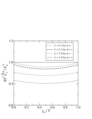
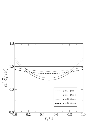
Figure 1: Left: the correlator $\widehat{\cal{C}}_{1}^{\sigma}(x_{0},y_{0})$ of eq. (5.3), normalised to the tree-level value (solid line). The time extent is $T=3.0\,{\rm fm}$, the quark mass $m=5\,{\rm MeV}$, the $x_{0}$-coordinate $x_{0}/T=-1/4$, the pion decay constant $F_{\pi}=93\,{\rm MeV}$, and the chiral condensate $\Sigma=(250\,{\rm MeV})^{3}$. Right: the same observable with the spatial extent $L=2.1\,{\rm fm}$, but in an ensemble with a fixed topological charge $\nu$.

The above results are obtained in a fixed $\theta$-vacuum. By performing a Fourier transform in $\theta$ one can obtain averages in sectors of “fixed topology”, characterised by an index $\nu$. In ref. [?] the special rôle of topology in the $\epsilon$-regime was emphasised, noting that certain quantities depend quite strongly on the index near the chiral limit. Recent developments in the understanding of the rôle of topology show that correlation functions in fixed topological sectors can be defined also in QCD [?,?]. Although this result is universal [?], different topological sectors can be identified through the index of the fermion operator only if fermionic discretisations with an exact chiral symmetry are used.

When considering averages in sectors of fixed $\nu$, poles in the quark mass $m$ are expected to occur in certain correlation functions. Whether or not such poles also appear in quantities considered here is what we discuss in the following. Note that in the regime of larger quark masses (conventionally called $p$-regime), topology does not play a major rôle, and it is commonplace to present predictions of ChPT for fixed $\theta$ rather than $\nu$.

The transition to sectors of fixed topology simply amounts to substituting $C_{\theta}(u/2)$ by $C_{\nu}(u/2)$, whose definition is specified in Appendix D. As can be seen from Fig. 1 (right panel) the time behaviour of the correlator is indeed strongly modified in the small-mass region. Although the correlators do not develop any poles for $m\to 0$ (because $C_{\nu}(u/2)$ is multiplied by $u$), their time dependence does not vanish in this limit, for $\nu\neq 0$.

So far we have ignored the correlation function $[\widehat{\cal{C}}_{2}^{\pm}]$. The reason is that it arises only at order $\epsilon^{8}$, owing to the fact that it contains two powers of the mass matrix each contributing a factor of order $\epsilon^{4}$. Actually, if a diagonal mass matrix and flavour assignments as in the derivation of eq. (5.3) are chosen, $[\widehat{\cal C}_{2}^{\pm}]$ vanishes identically. In order to isolate the “pure QCD” contribution to the $\Delta{I}=1/2$ enhancement at next-to-leading order, it is thus sufficient to concentrate on the LECs $g_{1}^{\pm}$, dropping the operator $[\widehat{\cal{O}}_{2}^{\pm}]_{\alpha\beta\gamma\delta}$ altogether.

The determination of $g_{1}^{+}$ and $g_{1}^{-}$ is greatly facilitated by considering suitable ratios of correlation functions. If we define

$$K^{\pm}(x_{0},y_{0})\equiv 2\frac{\widehat{\cal C}_{1}^{\pm}(x_{0},y_{0})}{{\cal C}^{aa^{\dagger}}(x_{0}){\cal C}^{bb^{\dagger}}(y_{0})},$$ (5.48)

choose $T^{a^{\dagger}}\equiv(T^{a})^{\dagger}$, $T^{b^{\dagger}}\equiv(T^{b})^{\dagger}$, with $T^{a},\,T^{b}$ as in eq. (D.132), and insert the expressions derived above we obtain

$$K^{\sigma}(x_{0},y_{0})=1+\frac{2\sigma}{F_{\pi}^{2}T^{2}}\rho^{3}\left\{\beta_{1}\rho^{-3/2}-k_{00}\right\},\quad\sigma=\pm.$$ (5.49)

Thus, at order $\epsilon^{2}$ the dependence on $m$, $x_{0}$, $y_{0}$ and — if the correlations are computed for fixed topology — also on $\nu$ drops out in the ratios $K^{\pm}$. If we write

$$K^{\sigma}(x_{0},y_{0})=1+\sigma R(x_{0},y_{0}),\quad\sigma=\pm,$$ (5.50)

we can plot the expression for $R(x_{0},y_{0})$ (which is independent of $x_{0},y_{0}$ at order $\epsilon^{2}$) as a function of the volume, see Fig. 2. Another important ratio is

$$H(x_{0},y_{0})\equiv\frac{\widehat{\cal C}_{1}^{-}(x_{0},y_{0})}{\widehat{\cal C}_{1}^{+}(x_{0},y_{0})}=\frac{K^{-}(x_{0},y_{0})}{K^{+}(x_{0},y_{0})}.$$ (5.51)

In terms of the one-loop correction $R(x_{0},y_{0})$ it is given at ${\rm O}(\epsilon^{2})$ by

$$H(x_{0},y_{0})=1-2R(x_{0},y_{0})=1-\frac{4}{F_{\pi}^{2}T^{2}}\rho^{3}\left\{\beta_{1}\rho^{-3/2}-k_{00}\right\},$$ (5.52)

and the right panel in Fig. 2 shows a plot of $H$ as a function of the volume for different geometries. The computation of the corresponding ratio of three-point functions in lattice QCD in the $\epsilon$-regime is then directly proportional to $g_{1}^{-}/g_{1}^{+}$:

$$\frac{g_{1}^{-}}{g_{1}^{+}}=\frac{k_{1}^{-}}{k_{1}^{+}}\frac{C_{1}^{-}(x_{0},y_{0})}{C_{1}^{+}(x_{0},y_{0})}\frac{1}{H(x_{0},y_{0})},$$ (5.53)

where

$$C_{1}^{\pm}(x_{0},y_{0})=\sum_{\vec{x},\vec{y}}\left\langle J_{0}(x)\,{\cal Q}_{1}^{\pm}(0)\,J_{0}(y)\right\rangle$$ (5.54)

is the three-point correlation function in QCD. Here it is assumed that the Wilson coefficients $k_{1}^{\pm}$ are known for the particular scheme in which the operators ${\cal Q}_{1}^{\pm}$ are renormalised.

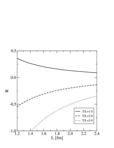
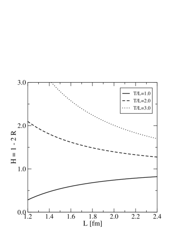
Figure 2: The quantities $R(x_{0},y_{0})$ (left panel) and $H(x_{0},y_{0})$ (right panel) plotted as functions of the box size and geometry. For $F$ we have here chosen a value indicated by quenched simulations at modest volumes, $F\approx 103\,{\rm MeV}$ [?], but the dependence of $R$ on $F$ is only through an overall factor $1/(FT)^{2}$ and the curves have thus the same form for any other value as well.

Let us stress that, in the main result of this section, eq. (5.52), the Goldstone zero-momentum mode contribution, $C_{\theta}(u/2)$ or $C_{\nu}(u/2)$, has cancelled completely at this order. This means that the result in the $\epsilon$-regime at NLO can be obtained from a NLO calculation of the same quantity in the $p$-regime, by taking just the leading term in a Taylor expansion in the pseudoscalar mass $m_{\rm P}^{2}\equiv 2m\Sigma/F^{2}$. Note that, as long as the volume is kept fixed, the contributions from non-zero modes are infrared-safe, since the chiral logarithms encountered in infinite volume are replaced by logarithms of the volume. The fact that the expression for the ratio $\widehat{\mathcal{C}}_{1}^{-}/\widehat{\mathcal{C}}_{1}^{+}$ in the $p$-regime can be Taylor-expanded in $m_{\rm P}^{2}$ for fixed volume can also be used in practice to obtain the result in the $\epsilon$-regime indirectly from numerical simulations in the $p$-regime, by fitting the numerically determined ratio $\widehat{\mathcal{C}}_{1}^{-}/\widehat{\mathcal{C}}_{1}^{+}$ to a constant (which is the result in the $\epsilon$-regime) plus ${{\rm O}}(m_{\rm P}^{2})$ corrections with some unknown coefficient.

5.4 The quenched approximation

Currently, numerical simulations of lattice QCD with Ginsparg-Wilson fermions are mostly restricted to the quenched approximation, owing to the large computational cost. Here we discuss the implications of quenching for our strategy.

Quenched QCD can be treated within the framework of an effective Lagrangian, with the resulting low-energy expansion referred to as quenched Chiral Perturbation Theory (qChPT) [?,?]. The theoretical status of qChPT is, however, questionable. This manifests itself in the occurrence of infrared divergences in certain correlation functions. These divergences reflect, at least partially, the sickness of quenched QCD. Here we adopt the pragmatic assumption that — despite the fact that it is not an asymptotic expansion of quenched QCD (for a fixed number of colours $N_{\rm c}$) — quenched ChPT does describe the low-energy regime of quenched QCD in certain ranges of kinematical scales, where correlation functions can be parameterised in terms of effective coupling constants, the latter being defined as the couplings which appear in the Lagrangian of the effective theory. Under this assumption we now discuss the determination of the counterparts of $g_{1}^{\pm}$ in the quenched theory, via the matching of correlation functions computed in quenched QCD and qChPT.

The main difference between ChPT considered in the quenched and unquenched theories is that in the former there is no decoupling of flavour singlets from the pseudo-Goldstone bosons. The dynamics of the singlet field $\Phi_{0}$ must then be incorporated into the effective chiral Lagrangian, which requires additional LECs associated with the new interaction terms. To be more precise, we consider the quenched effective Lagrangian in the so-called “replica formalism” [?,?]

$${\cal L}_{\rm E}^{\rm quen} = {\textstyle\frac{1}{4}}F^{2}\,{\rm Tr}\left[(\partial_{\mu}U)\partial_{\mu}U^{-1}\right]-{\textstyle\frac{1}{2}}\Sigma\,{\rm Tr}\left[U_{\theta}UM^{\dagger}+MU^{-1}U_{\theta}^{-1}\right]$$ (5.55)

$$+\frac{m_{0}^{2}}{2N_{\rm c}}\Phi_{0}^{2}+\frac{\alpha}{2N_{\rm c}}(\partial_{\mu}\Phi_{0})^{2}.$$

In the replica method one introduces $N_{\rm v}$ valence quarks that are considered independently from the number of sea quarks, $N_{\rm f}$, which will eventually be taken to zero. In the quenched case the fields $U$ are promoted from elements of SU($N_{\rm f}$) to those of U($N_{\rm f}$). The factor $U_{\theta}$ is given by $U_{\theta}=\exp(i\theta I_{N_{\rm v}}/N_{\rm v})$, where $I_{N_{\rm v}}$ is the unit matrix in the subspace corresponding to valence quarks. In addition to the LECs $F$ and $\Sigma$ (which, of course, may differ from those in the full theory), there are new parameters, $\alpha$ and $m_{0}$, which are associated with the singlet field $\Phi_{0}$.

We have noted above that poles in the quark mass may appear in fermion propagators if the theory is considered for fixed non-trivial topology. These poles are expected to be the same in the full and quenched cases. For fixed topology, the counting rules of the $\epsilon$-expansion remain unchanged when passing to the quenched theory.

When the $\Delta{S}=1$ weak interactions are incorporated into the quenched setting, the larger symmetry group and the presence of the singlet field $\Phi_{0}$ may allow for additional interactions that need to be taken into account at a given order of the chiral expansion. Without going into further detail, we note that the current ${\cal J}_{\mu}^{a}$ and the operators ${\cal O}_{1}$ and ${\cal O}_{2}$ need not be modified in the quenched case, provided that an additional expansion in $1/N_{\rm c}$ is assumed, which is needed in order to justify the truncation in operators involving higher powers of $\Phi_{0}$. This truncation has also been invoked to arrive at eq. (5.55). Furthermore, the effective weak Hamiltonian does not have to be supplemented by additional operators. The classification of operators according to the valence symmetry does not give rise to ambiguities like those discussed in [?] for operators that appear in the conventional SU(3)-case. The argument which proves the absence of these ambiguities is analogous to the one discussed in [?] for the 27-plet operator in the SU(3) case. We refer the reader to this reference for more details.

We now give the expressions for the quenched analogues of the correlation functions in eqs. (5.46) and (5.3) for fixed topology. They are formally obtained by taking $N_{\rm f}\to 0$ in the general expressions for the correlators obtained from the Lagrangian in eq. (5.55). For the two-point function this yields [?,?]

$${\cal C}^{ab;\rm quen}(x_{0})={\rm Tr}(T^{a}T^{b})\frac{F^{2}}{2T}\left\{1+\frac{1}{F^{2}T^{2}}\rho^{3}\Big{[}uC_{\nu}^{\rm quen}(u/2)\,h_{1}(x_{0}/T)\Big{]}\right\},$$ (5.56)

where

$$C_{\nu}^{\rm quen}=\frac{1}{N_{\rm v}}\left\langle{\rm Re}\,{\rm Tr}_{\rm v}U_{0}\right\rangle_{\nu,U_{0}}$$ (5.57)

and ${\rm Tr}_{\rm v}$ denotes the trace over the valence subgroup. The precise meaning of the average $\langle{\rm Re}\,{\rm Tr}_{\rm v}U_{0}\rangle_{\nu,U_{0}}$ is specified in [?]. Note that there is no dependence on the singlet couplings $m_{0}^{2}$ and $\alpha$. As a result, it is easy to see that the quenched results can be simply obtained from the unquenched expressions in the limit $N_{\rm f}\to 0$. In a similar manner one finds the result for the three-point function

$$\widehat{\cal C}_{1}^{\sigma;{\rm quen}}(x_{0},y_{0}) = \frac{F^{4}}{8T^{2}}\bigg{\{}1+\frac{1}{F^{2}T^{2}}\rho^{3}\Big{[}2\sigma(\beta_{1}\rho^{-3/2}-k_{00})$$

$$\phantom{-\frac{F_{\pi}^{4}}{8T^{2}}\bigg{\{}1+\frac{1}{F_{\pi}^{2}T^{2}}\rho^{3}\Big{[}}+uC_{\nu}^{\rm quen}(u/2)\Big{(}h_{1}(x_{0}/T)+h_{1}(y_{0}/T)\Big{)}\Big{]}\bigg{\}}.\phantom{FF}$$

One can easily see that the ratios $K^{\pm}(x_{0},y_{0})$ and $H(x_{0},y_{0})$ defined above remain unchanged, and thus the relation in eq. (5.53) between the ratio $g_{1}^{-}/g_{1}^{+}$ and the correlation functions carries over to the quenched case without modification, at this order. The same is true for the expansion of the ratio $\widehat{\cal{C}}_{1}^{-}/\widehat{\cal{C}}_{1}^{+}$ in $m_{\rm P}^{2}$ at fixed volume, which was discussed at the end of Sect. 5.3.

6 Decoupling of the charm quark in Chiral Perturbation Theory

We will now depart from the unphysical situation of a charm quark degenerate with the other light quarks and investigate its effects in the framework of ChPT. In particular, we will show how the $\Delta{I}=1/2$ and 3/2 amplitudes evolve as $m_{c}$ is increased, but stays below the QCD scale, in order for ChPT to remain applicable. The aim is to find a relation between the LECs $g_{1}^{\pm}$ and the corresponding couplings in the theory where the charm quark has been integrated out. Here we only sketch the procedure and state the main results: a detailed account of the calculation is given in a separate publication [?].

6.1 Basic setup

The effective Lagrangian ${\cal L}_{\rm E}$ of QCD with an $\rm SU(4)_{L}\times SU(4)_{R}$ chiral symmetry was defined to leading order in eq. (5.31). Since the decoupling of the charm quark is insensitive to infrared physics, we will, for simplicity, consider the theory in infinite volume. Unlike the situation encountered in the $\epsilon$-regime, counterterms must then be added to the effective Lagrangian, if higher orders in the expansion are considered. For our purposes it is sufficient to include the counterterm

$$\delta{\cal L}_{\rm E}=L_{4}\,{\rm Tr}[\partial_{\mu}U\partial_{\mu}U^{\dagger}]{\rm Tr}[\chi^{\dagger}U+U^{\dagger}\chi],$$ (6.59)

where the vacuum angle $\theta$ has been set equal to zero and $\chi$ is defined as

$$\chi=\frac{2\Sigma M}{F^{2}}.$$ (6.60)

Phenomenological estimates for the value of $L_{4}$ are available in the physical $\rm SU(3)_{L}\times SU(3)_{R}$-symmetric case [?,?].

Weak interactions are incorporated through the effective Hamiltonian, which, at leading order, contains the operators ${\cal O}_{1}$ and ${\cal O}_{2}$ given in eqs. (5.36) and (5.37). We now consider a mass matrix of the form

$$M={\rm diag}(m_{u},m_{d},m_{s},m_{c})$$ (6.61)

with $m_{c}\gg m_{u}=m_{d}=m_{s}$, noting that the restriction to degenerate non-charm quarks is irrelevant for our purposes. Furthermore we define

$$\chi_{uu}\equiv\frac{2m_{u}\Sigma}{F^{2}},\quad\chi_{cc}\equiv\frac{2m_{c}\Sigma}{F^{2}}.$$ (6.62)

If momenta $p$ with $p^{2}\;\raisebox{-2.58334pt}{$\stackrel{{\scriptstyle\textstyle{>}}}{{\sim}}$}\;\chi_{cc}$ are excluded, then one expects the physics of the SU(4)-symmetric theory to be described by another effective Lagrangian from which the heavy scale has been integrated out, and which possesses an $\rm SU(3)_{L}\times SU(3)_{R}$ chiral symmetry. Our task is now to derive the effective weak Hamiltonian of such a theory, assuming that the LECs $g_{1}^{\pm}$ are already known in the SU(4)-symmetric case. In order to define our power-counting rules we assume the following hierarchies:

$$\chi_{uu}\ll\chi_{cc}\ll(4\pi F)^{2}.$$ (6.63)

In accordance with these relations, we work at order $\chi_{cc}/(4{\pi}F)^{2}$ in the chiral expansion, while dropping all terms of order $\chi_{uu}/\chi_{cc}$ and $\chi_{uu}/(4{\pi}F)^{2}$.

The form of the strong interaction part of the effective $\rm SU(3)_{L}\times SU(3)_{R}$ theory is identical to ${\cal L}_{\rm E}$, but formulated in terms of SU(3) matrices and modified LECs. In order to distinguish them from their counterparts in the $\rm SU(4)_{L}\times SU(4)_{R}$-symmetric theory, we will denote them with a bar. The effective action then reads

$$\bar{\cal L}_{\rm E}={\textstyle\frac{1}{4}}\bar{F}^{2}\,{\rm Tr}\left[(\partial_{\mu}\bar{U})\partial_{\mu}\bar{U}^{\dagger}\right]-{\textstyle\frac{1}{2}}\bar{\Sigma}\,{\rm Tr}\left[\bar{U}\bar{M}^{\dagger}+\bar{M}\bar{U}^{\dagger}\right],$$ (6.64)

where $\bar{U}\in\rm SU(3)$ and

$$\bar{M}={\rm diag}(m_{u},m_{d},m_{s}).$$ (6.65)

Flavour indices are denoted by $\bar{\alpha},\bbeta,\ldots$ and take their values from the set $(u,d,s)$. The construction of non-singlet weak operators transforming under ${\bf{3}}^{*}\otimes{\bf{3}}^{*}\otimes{\bf{3}}\otimes{\bf{3}}$ of $\rm SU(3)_{L}$ proceeds along the same lines as in the SU(4)-case. By considering the power-counting rules introduced above, one finds that the SU(3)-counterpart of ${\cal O}_{2}$ is of relative order $(\chi_{uu}/\chi_{cc})^{2}$ and can thus be dropped. This leaves

$${[\bar{\cal O}_{1}]}_{\bar{\alpha}\bbeta\bar{\gamma}\bar{\delta}} \equiv {\textstyle\frac{1}{4}}\bar{F}^{4}\left(\bar{U}\partial_{\mu}\bar{U}^{\dagger}\right)_{\bar{\gamma}\bar{\alpha}}\left(\bar{U}\partial_{\mu}\bar{U}^{\dagger}\right)_{\bar{\delta}\bbeta}$$ (6.66)

$${[\bar{\cal O}_{3}]}_{\bar{\alpha}\bar{\gamma}} \equiv {\textstyle\frac{1}{2}}\bar{F}^{2}\bar{\Sigma}\big{(}\bar{U}\bar{M}^{\dagger}+\bar{M}\bar{U}^{\dagger}\big{)}_{\bar{\gamma}\bar{\alpha}},$$ (6.67)

and the effective weak Hamiltonian, denoted by $\bar{\cal{H}}_{\rm{w}}^{\rm ChPT}$, is a combination of these two operators. The matching proceeds by enforcing equality between correlation functions involving left-handed flavour currents. In analogy with the procedure outlined in Sect. 5.1, the latter are derived by defining covariant derivatives according to

$$\partial_{\mu}{U}\to D_{\mu}{U}\equiv(\partial_{\mu}+iA_{\mu}^{a}\bar{T}^{a})U,\qquad\partial_{\mu}\bar{U}\to D_{\mu}\bar{U}\equiv(\partial_{\mu}+iA_{\mu}^{a}\bar{T}^{a})\bar{U},$$ (6.68)

where $\bar{T}^{a}$ are the Hermitian generators of SU(3). The left-handed currents ${\cal{J}}_{\mu}^{a}$ and $\bar{\cal{J}}_{\mu}^{a}$ in the SU(4)- and SU(3)-symmetric theories are then obtained by taking functional derivatives with respect to $A_{\mu}^{a}$.

In order to perform the matching to leading order in the weak Hamiltonian we require

$$\left\langle{\cal J}_{\mu}^{a}(x){\cal J}_{\nu}^{b}(y)\right\rangle_{\rm SU(4)} = \left\langle\bar{\cal J}_{\mu}^{a}(x)\bar{\cal J}_{\nu}^{b}(y)\right\rangle_{\rm SU(3)},$$ (6.69)

$$\left\langle{\cal J}_{\mu}^{a}(x){\cal H}_{\rm w}^{\rm ChPT}(z){\cal J}_{\mu}^{b}(y)\right\rangle_{\rm SU(4)} = \left\langle\bar{\cal J}_{\mu}^{a}(x)\bar{\cal H}_{\rm w}^{\rm ChPT}(z)\bar{\cal J}_{\mu}^{b}(y)\right\rangle_{\rm SU(3)},$$ (6.70)

where the expectation values are evaluated using the strangeness conserving Lagrangian, and it is understood that space-time separations are large compared with the scales set by $\chi_{cc}$ and $4{\pi}F$. The objective is then to compute the observables on the left-hand sides of eqs. (6.69) and (6.70) to the order in $\chi_{cc}$ defined previously and find out how the LECs and operators on the right-hand sides must be adjusted.

6.2 Matching of the SU(3) and SU(4)-symmetric theories

By enforcing the matching condition on current-current correlators one obtains the relations between the low-energy parameters $F$ and $\bar{F}$, as well as $\Sigma$ and $\bar{\Sigma}$. Here we omit all the details of the calculation and refer to [?]. At one-loop level, the pion decay constant in the chiral limit in the SU(3)-symmetric theory, $\bar{F}$, is related to $F$ via

$$\bar{F}^{2}=F^{2}\left\{1-\frac{1}{2}\frac{\chi_{cc}}{(4{\pi}F)^{2}}\Big{[}\ln\frac{\chi_{cc}}{2\bar{\mu}^{2}}-1-16(4\pi)^{2}L_{4}^{\rm\overline{MS\kern-0.35002pt}\kern 0.35002pt}\Big{]}\right\}.$$ (6.71)

Here we have adopted the conventions of the ${\rm\overline{MS\kern-0.50003pt}\kern 0.50003pt}$-scheme, with $\bar{\mu}$ denoting the subtraction scale. A similar relation can be derived for the parameters $\Sigma$ and $\bar{\Sigma}$ [?].

When matching the effective weak Hamiltonians according to eq. (6.70), it is convenient to replace ${\cal{H}}_{\rm{w}}^{\rm ChPT}(z)$ by the operator ${\cal{O}}_{1}$ in the ${\rm SU(4)_{L}\times SU(4)_{R}}$ theory and work out the set of operators in the ${\rm SU(3)_{L}\times SU(3)_{R}}$ theory it leads to. Skipping over the details of the calculation, we simply quote the result: when moving from ${\cal{H}}_{\rm{w}}^{\rm ChPT}$ to $\bar{\cal H}_{\rm w}^{\rm ChPT}$, the operator $[{\cal{O}}_{1}]$ must be replaced by

$$[{\cal{O}}_{1}]_{\alpha\beta\gamma\delta} \longrightarrow c_{1}[\bar{\cal{O}}_{1}]_{\bar{\alpha}\bbeta\bar{\gamma}\bar{\delta}}+c_{2}\Big{(}\delta_{{\alpha}c}\delta_{{\delta}c}[\bar{\cal{O}}_{1}]_{\bbeta\bar{\kappa}\bar{\kappa}\bar{\gamma}}+\delta_{{\beta}c}\delta_{{\gamma}c}[\bar{\cal{O}}_{1}]_{\bar{\alpha}\bar{\kappa}\bar{\kappa}\bar{\delta}}\Big{)}$$ (6.72)

$$+d_{2}\Big{(}\delta_{{\alpha}c}\delta_{{\delta}c}[\bar{\cal{O}}_{3}]_{\bbeta\bar{\gamma}}+\delta_{{\beta}c}\delta_{{\gamma}c}[\bar{\cal{O}}_{3}]_{\bar{\alpha}\bar{\delta}}\Big{)},$$

where the coefficients $c_{1},c_{2}$ and $d_{2}$ are given by

$$c_{1}=1+2K\frac{\chi_{cc}}{F^{2}},$$ (6.73)

$$c_{2}=-\frac{3}{4}\frac{\chi_{cc}}{(4\pi F)^{2}}\ln\frac{\Lambda_{\chi}^{2}}{\chi_{cc}},\qquad d_{2}=-\frac{1}{2}\frac{\chi_{cc}}{(4\pi F)^{2}}\ln\frac{\Lambda_{\chi}^{2}}{\chi_{cc}},$$ (6.74)

and SU(3) singlet structures have been omitted in eq. (6.72). Here $\Lambda_{\chi}$ is some physical scale that will in general be different for $c_{2}$ and $d_{2}$, since it incorporates the effect of the finite corrections (similar to the terms proportional to $L_{4}^{\rm\overline{MS\kern-0.35002pt}\kern 0.35002pt}$ in eq. (6.71), but for the weak interaction part [?]) that have not been included in this case. On the other hand, $K$ denotes a particular such coupling that could contribute at this order through the higher-dimensional operator

$$\frac{K}{F^{2}}[{\cal{O}}_{1}]_{\bar{\alpha}\bbeta\bar{\gamma}\bar{\delta}}{\rm Tr}\big{[}\chi^{\dagger}U+U^{\dagger}\chi\big{]}.$$ (6.75)

Since this operator is of order $\chi_{cc}/F^{2}$ it must be included according to our power counting rules. Thus we find that $c_{2}$ and $d_{2}$ contain a logarithmic enhancement in $m_{c}$, while $c_{1}$ does not.

A weak operator $[{\cal O}_{2}]_{\bar{\alpha}\bbeta\bar{\gamma}\bar{\delta}}$ of the form shown in eq. (5.37) can also contribute to the effective weak Hamiltonian $\bar{\cal H}_{\rm w}^{\rm ChPT}$. For our choice of mass matrix and the adopted power counting scheme, there is indeed a tree-level effect of the form

$$-\frac{m_{c}^{2}}{F^{2}}\Big{(}\delta_{{\alpha}c}\delta_{{\delta}c}[\bar{\cal{O}}_{3}]_{\bbeta\bar{\gamma}}+\delta_{{\beta}c}\delta_{{\gamma}c}[\bar{\cal{O}}_{3}]_{\bar{\alpha}\bar{\delta}}\Big{)},$$ (6.76)

which is of order $m_{c}^{2}$. In the region of small $m_{c}$ this is parametrically smaller than the term with the same structure in eq. (6.72), which is multiplied by $d_{2}$. As the latter is formally of order $m_{c}$, we drop the above contribution from now on.

We are now in a position to work out the effective weak Hamiltonian in the ${\rm SU(3)_{L}\times SU(3)_{R}}$ theory. To this end we start with the expression for ${\cal{H}}_{\rm w}^{\rm ChPT}$ in the SU(4)-symmetric theory, eq. (5.38), drop the contribution from ${\cal{O}}_{2}$ for the reason just mentioned, and write the remaining terms in the form

$${\cal H}_{\rm w}^{\rm ChPT}=\frac{g^{2}_{\rm{w}}}{2M_{W}^{2}}(V_{us})^{*}V_{ud}\sum_{\sigma=\pm}g_{1}^{\sigma}c_{\alpha\beta\gamma\delta}(P_{2}^{\sigma}\,P_{1}^{\sigma})_{\alpha\beta\gamma\delta;\lambda\nu\rho\tau}[{\cal{O}}_{1}]_{\lambda\nu\rho\tau},$$ (6.77)

where the projectors $P_{1}^{\sigma}$ and $P_{2}^{\sigma}$ are defined in eqs. (A.95) and (A.96). From the above discussion we know that, to leading order in $m_{c}$, the matching is achieved by replacing ${\cal{O}}_{1}$ by the right-hand side of eq. (6.72), with the coefficients $c_{1},\,c_{2}$ and $d_{2}$ specified as above. The expression for $\bar{\cal{H}}_{\rm w}^{\rm ChPT}$ is obtained by inserting eq. (6.72) into eq. (6.77) and performing the decomposition into irreducible representations of SU(3). The resulting expression for $\bar{\cal{H}}_{\rm{w}}^{\rm ChPT}$ is rather lengthy, and here we simply quote the result for the physical choice of flavours, characterised by $c_{suud}=1$ and $c_{sccd}=-1$:

$$\bar{\cal{H}}_{\rm w}^{\rm ChPT} = \frac{g_{\rm w}^{2}}{2M_{W}^{2}}(V_{us})^{*}V_{ud}\,\bigg{\{}c_{1}g_{1}^{+}[\widehat{\bar{\cal{O}}}_{1}^{+}]_{suud}+\left(\frac{c_{1}-5c_{2}}{5}g_{1}^{+}+(c_{1}-c_{2})g_{1}^{-}\right)[\bar{\cal{R}}_{1}^{+}]_{sd}$$ (6.78)

$$\phantom{\frac{g_{\rm w}^{2}}{2M_{W}^{2}}(V_{us})^{*}V_{ud}\,}-\frac{d_{2}}{2}(g_{1}^{+}+g_{1}^{-})[\widehat{\bar{\cal{O}}}_{3}]_{sd}\bigg{\}}.$$

In this expression the operators $[\widehat{\bar{\cal{O}}}_{1}^{+}]_{suud}$ and $[\bar{\cal{R}}_{1}^{+}]_{sd}$ are defined as

$$[\widehat{\bar{\cal{O}}}_{1}^{+}]_{suud} = {\textstyle\frac{1}{2}}\left([\bar{\cal{O}}_{1}]_{suud}+[\bar{\cal{O}}_{1}]_{sudu}-{\textstyle\frac{1}{5}}[\bar{\cal{O}}_{1}]_{s{\bar{\kappa}\bar{\kappa}}d}\right)={\textstyle\frac{3}{5}}\left([\bar{\cal{O}}_{1}]_{sudu}+{\textstyle\frac{2}{3}}[\bar{\cal{O}}_{1}]_{suud}\right),$$ (6.79)

$${[\bar{\cal{R}}_{1}^{+}]_{sd}} = {\textstyle\frac{1}{2}}[\bar{\cal{O}}_{1}]_{s{\bar{\kappa}\bar{\kappa}}d}.$$ (6.80)

The operator $[\widehat{\bar{\cal{O}}}_{1}^{+}]_{suud}$ transforms under the irreducible representation of dimension 27 of SU(3), and in eq. (6.79) we have listed two equivalent forms which are found in the literature. The operators $[\bar{\cal{R}}_{1}^{+}]_{sd}$ and $[\widehat{\bar{\cal{O}}}_{3}]_{sd}$ both transform under the 8-dimensional irreducible representation.

After inserting the expressions for the coefficients $c_{1},\,c_{2}$ and $d_{2}$ while keeping only logarithmic terms we finally arrive at

$$\bar{\cal{H}}_{\rm w}^{\rm ChPT} = \frac{g_{\rm w}^{2}}{2M_{W}^{2}}(V_{us})^{*}V_{ud}\,\Bigg{\{}g_{1}^{+}[\widehat{\bar{\cal{O}}}_{1}^{+}]_{suud}$$ (6.81)

$$+\left[\frac{1}{5}g_{1}^{+}\bigg{(}1+\frac{15}{4}\frac{\chi_{cc}}{(4\pi F)^{2}}\ln\frac{\Lambda_{\chi}^{2}}{\chi_{cc}}\bigg{)}+g_{1}^{-}\bigg{(}1+\frac{3}{4}\frac{\chi_{cc}}{(4\pi F)^{2}}\ln\frac{\Lambda_{\chi}^{2}}{\chi_{cc}}\bigg{)}\right][\bar{\cal{R}}_{1}^{+}]_{sd}$$

$$+\bigg{[}\frac{1}{4}(g_{1}^{+}+g_{1}^{-})\frac{\chi_{cc}}{(4\pi F)^{2}}\ln\frac{\Lambda_{\chi}^{2}}{\chi_{cc}}\bigg{]}[\widehat{\bar{\cal{O}}}_{3}]_{sd}\Bigg{\}}.$$

This result illustrates the effects of the decoupling of the charm quark. One observes that the coefficients of the octet part (i.e. the last two lines) contain an extra logarithmic factor, $\chi_{cc}\ln\Lambda_{\chi}^{2}/\chi_{cc}$, which for $\chi_{cc}\ll\Lambda_{\chi}^{2}$ is parametrically larger than the coefficient of the 27-plet (first line), even if the linear term of eq. (6.73) were kept in the latter. It is well known that the octet part only mediates $\Delta{I}=1/2$ transitions, whereas the 27-plet contains both $\Delta{I}=3/2$ and 1/2 contributions. Thus, the logarithmic terms in front of the octet operators describe the departure of the $\Delta{I}=1/2$ amplitude from the SU(4)-symmetric situation.

We stress that these findings apply to the case of a moderately heavy charm quark, which must be light enough for ChPT to be valid. Whether or not the observed enhancement survives if the charm quark is tuned towards its physical value must be studied in a lattice simulation.

7 Numerical results in the SU(4)-symmetric theory

We now describe the findings of our numerical investigations in the theory with a light, degenerate charm quark, i.e. $m_{u}=m_{d}=m_{s}=m_{c}$. Thereby we will gain information as to what extent physics at the intrinsic QCD scale of a few hundred MeV contributes to the enhancement of the $\Delta{I}=1/2$ amplitude. The effects of a heavier charm quark will be the subject of future investigations.

In our numerical work we have used the quenched approximation, whose deficits in this context have been discussed in Sect. 5. Although one may call into question any physical interpretation of quenched numerical data, we regard the work presented here primarily as a study to yield valuable information for future simulations.

7.1 General definitions

Our task is the determination of the low-energy constants $g_{1}^{+}$ and $g_{1}^{-}$. Of particular interest is the ratio $g_{1}^{-}/g_{1}^{+}$, which, according to eq. (5.40), determines the ratio of amplitudes $A_{0}/A_{2}$ at leading order in ChPT. The determination of LECs proceeds as usual, by computing suitable correlation functions in simulations of lattice QCD and fitting the results to the expressions obtained in ChPT. At non-vanishing lattice spacing such a procedure is justified only if a fermionic discretisation is chosen which preserves chiral symmetry. Here we have used the Neuberger-Dirac operator, which was already discussed briefly in Sect. 3.1.

From the previous sections of this paper it is clear that we are particularly interested in correlation functions of left-handed currents and four-quark operators. More specifically, we define the non-singlet left-handed current as

$$[J_{\mu}(x)]_{\alpha\beta}=(\overline{\psi}_{\alpha}\gamma_{\mu}P_{-}\widetilde{\psi}_{\beta})(x),$$ (7.82)

where $\alpha,\,\beta$ denote generic flavour indices, and the modified quark field $\widetilde{\psi}$ is given in eq. (3.21). Our earlier considerations show that we can concentrate on the operator ${\cal{Q}}_{1}^{\pm}$, whose definition we repeat here:

$${\cal Q}_{1}^{\pm}=\Big{\{}(\overline{s}\gamma_{\mu}P_{-}\tilde{u})(\overline{u}\gamma_{\mu}P_{-}\tilde{d})\pm(\overline{s}\gamma_{\mu}P_{-}\tilde{d})(\overline{u}\gamma_{\mu}P_{-}\tilde{u})\Big{\}}-(u\,{\to}\,c).$$ (7.83)

We then consider the following two-point and three-point correlators:

$$C(x_{0}) = \sum_{\vec{x}}\left\langle[J_{0}(x)]_{\alpha\beta}[J_{0}(0)]_{\beta\alpha}\right\rangle,$$ (7.84)

$$C_{1}^{\pm}(x_{0},y_{0}) = \sum_{\vec{x},\vec{y}}\left\langle[J_{0}(x)]_{du}\,[{\cal{Q}}_{1}^{\pm}(0)]\,[J_{0}(y)]_{us}\right\rangle.$$ (7.85)

After performing the Wick contractions, the correlators can be expressed in terms of the quark propagator $S(x,y)$,

$${S}_{\alpha}(x,y)\equiv\left\langle\widetilde{\psi}_{\alpha}(x)\overline{\psi}_{\alpha}(y)\right\rangle=\left\{(1-{\textstyle\frac{1}{2}}\bar{a}D)D_{m_{\alpha}}^{-1}\right\}(x,y),$$ (7.86)

where

$$D_{m_{\alpha}}=(1-{\textstyle\frac{1}{2}}\bar{a}m_{\alpha})D+m_{\alpha}$$ (7.87)

is the massive Neuberger-Dirac operator with bare mass $m_{\alpha}$. The left-handed propagator is then given by [?]

$$P_{-}{S}_{\alpha}(x,y)P_{+}=(1-{\textstyle\frac{1}{2}}\bar{a}m_{\alpha})^{-1}\left\{P_{-}(\gamma_{5}D_{m_{\alpha}})^{-1}P_{+}\right\}(x,y).$$ (7.88)

Since here we restrict ourselves to studying the case where all quark masses are degenerate, we will omit from now on the flavour label on propagators. The expression for the two-point function $C(x_{0})$ then reads

$$C(x_{0})=\sum_{\vec{x}}\left\langle{\rm Tr}\left\{\gamma_{0}P_{-}S(x,0)^{\dagger}P_{+}\gamma_{0}P_{-}S(x,0)P_{+}\right\}\right\rangle.$$ (7.89)

Turning now to the three-point correlator, we show in Fig. 3 the two types of diagrams that are obtained after performing the Wick contractions. An important consequence of restricting to the SU(4)-symmetric case is the fact that contributions from the so-called “Eye”-diagram vanish identically. Thus, only diagrams of the “Figure-8” type must be considered, and the expression for $C_{1}^{\pm}$ in terms of quark propagators becomes

$$C_{1}^{\pm}(x_{0},y_{0}) = \sum_{\vec{x},\vec{y}}\sum_{\mu=0}^{3}\Big{\{}\Big{\langle}{\rm Tr}\{\gamma_{\mu}P_{-}S(x,0)^{\dagger}\gamma_{0}P_{-}S(x,0)\}{\rm Tr}\{\gamma_{\mu}P_{-}S(y,0)^{\dagger}\gamma_{0}P_{-}S(y,0)\}\Big{\rangle}$$ (7.90)

$$\phantom{\sum}\mp\Big{\langle}{\rm Tr}\{\gamma_{\mu}P_{-}S(x,0)^{\dagger}\gamma_{0}P_{-}S(x,0)\gamma_{\mu}P_{-}S(y,0)^{\dagger}\gamma_{0}P_{-}S(y,0)\}\Big{\rangle}\Big{\}}.$$

Thus, correlation functions of operators which transform under irreducible representations of dimensions 84 and 20 are obtained by taking appropriate linear combinations of colour-connected and colour-disconnected contractions. As an aside we remark that the correlator $C_{1}^{+}(x_{0},y_{0})$ can also be used to compute the $B$-parameter $B_{K}$.

Figure 3: (a): the “Figure-8” diagram; (b): the “Eye” diagram. A grey circle denotes the insertion of ${\cal{Q}}_{1}^{\pm}$. The left-handed current is inserted at the black circles.

In accordance with the relation between ${\cal{Q}}_{1}^{\pm}$ and ${\cal{O}}_{1}$ (see eq. (A.101)), we note that the combination $k_{1}^{\pm}C_{1}^{\pm}(x_{0},y_{0})$ corresponds to $2g_{1}^{\pm}\hat{\cal C}_{1}^{\pm}(x_{0},y_{0})$ in the low-energy description, while $k_{1}^{\pm}C_{1}^{\pm}(x_{0},y_{0})/[C(x_{0})C(y_{0})]$ corresponds to $g_{1}^{\pm}K^{\pm}(x_{0},y_{0})$ (see eqs. (5.44) and (5.48)).

7.2 Technical details

In order to evaluate the correlation functions defined above, we have computed left-handed quark propagators on quenched background gauge configurations, using the Neuberger-Dirac operator with $s=0.4$ (see eq. (3.18)). We have employed the numerical techniques described in ref. [?], including the approximation of the inverse square root in $D$ by a minmax polynomial, the determination of the index $\nu$ of a given gauge configuration via the counting of zero modes, and the computation of a number of low modes of $P_{\sigma}D^{\dagger}DP_{\sigma}$, where $P_{\sigma}$ projects onto the chirality sector without zero modes. The calculation of the left-handed propagator was accelerated using low-mode preconditioning as described in [?]. Furthermore, the calculation was arranged such that the necessary Conjugate Gradient inversions were always performed in the chirality sector without zero modes.

In several recent publications [?,?] it was reported that correlation functions of left-handed currents show strong statistical fluctuations if the quark mass becomes of order $({\Sigma}V)^{-1}$ or smaller. The origin of these fluctuations could be traced to the low modes of the Dirac operator. For instance, if $m\simeq({\Sigma}V)^{-1}$ the contributions of a few eigenmodes to a given observables can be substantial, and the intrinsic space-time fluctuations of the eigenmodes then induce a large variance in the Monte Carlo estimate. In ref. [?] we proposed an exact technique which is able to reduce these fluctuations significantly, and which involves taking volume averages of the contributions of a certain number of low modes, $n_{\rm low}$, to the respective correlators. This technique, dubbed “low-mode averaging”, allows for the computation of two-point functions with controlled statistical errors in all topological sectors if $n_{\rm low}\;\raisebox{-2.58334pt}{$\stackrel{{\scriptstyle\textstyle{<}}}{{\sim}}$}\;7$, for quark masses around $m\sim(\Sigma V)^{-1}$. We note, though, that our technique cannot cure the fluctuations caused by extremely small eigenvalues of $D$, which are expected to occur with a non-negligible probability if $m\ll(\Sigma V)^{-1}$. As already remarked in [?], the solution to this problem may require the incorporation of the low-mode contribution to a particular observable into the importance sampling process.

For this study we extended the technique of low-mode averaging to the three-point functions corresponding to the diagrams in Fig. 3. It turned out, however, that low-mode averaging for three point functions requires a more careful tuning of its free parameters, in order to observe a significant reduction of statistical errors. Preliminary results of a detailed study have shown that masses $m\leq(\Sigma V)^{-1}$ can be reached if the number of low modes treated exactly is increased by a factor $2-3$ compared to the values in ref. [?]. For the purpose of this paper we have, instead, focused our attention on moderately light quark masses, corresponding to the $p$-regime. The parameters of our simulations are listed in Table 1.

Lattice	$\beta$	$L/a$	$T/a$	$n_{\rm{low}}$	$L[{\rm fm}]$	configs.
A	6.0	12	40	7	1.12	751
B	5.8485	12	30	5	1.49	638

Table 1: Simulation parameters, including the spatial and temporal lattice sizes, the number of low modes of the Dirac operator which are treated exactly, and the number of gauge configurations.

Lattice	$am$	$am_{\rm P}$	$aF_{\rm P}$	$C_{1}^{-}/C_{1}^{+}$
A	0.030	0.2248(30)	0.03434(37)	2.	46(40)
	0.040	0.2522(28)	0.03527(36)	1.	94(25)
	0.050	0.2772(27)	0.03623(36)	1.	67(18)
	0.060	0.3005(26)	0.03719(37)	1.	52(15)
	0.070	0.3224(27)	0.03815(39)	1.	41(12)
B	0.040	0.2628(28)	0.04149(45)	2.	03(25)
	0.053	0.2964(28)	0.04244(46)	1.	75(17)
	0.066	0.3268(28)	0.04339(47)	1.	57(12)
	0.078	0.3529(27)	0.04426(48)	1.	45(10)
	0.092	0.3816(27)	0.04527(49)	1.	35(8)

Table 2: Results for pseudoscalar meson masses and the ratio of three-point functions $C_{1}^{-}/C_{1}^{+}$ at several values of the bare quark mass.

7.3 Results

In order to determine pseudoscalar masses and decay constants we fitted the two-point function $C(x_{0})$ to the expression [?]

$$C(x_{0})={\textstyle\frac{1}{2}}m_{\rm P}F_{\rm P}^{2}\,\frac{\cosh\big{[}(T/2-|x_{0}|)m_{\rm P}\big{]}}{2\sinh[Tm_{\rm P}/2]}.$$ (7.91)

For lattice A these fits were performed for timeslices in the range $7\leq x_{0}/a\leq 19$, while for lattice B we used $7\leq x_{0}/a\leq 14$. The results are listed in Table 2. We note that the values obtained on lattice A for bare masses $am=0.04$ and 0.06 can be directly compared with ref. [?], where a larger spatial volume corresponding to $L=1.49\,{\rm fm}$ was used. The results for the pseudoscalar decay constant agree within errors, while the pseudoscalar meson mass at $am=0.040$ is larger by 4% (1.8$\sigma$) on the smaller spatial volume, which indicates a small finite-volume effect in the pseudoscalar correlator.

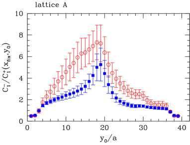
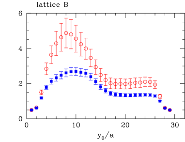
Figure 4: The ratio $C_{1}^{-}(x_{\rm fix},y_{0})/C_{1}^{+}(x_{\rm fix},y_{0})$ as a function of $y_{0}/a$ for lattices A (left panel) and B (right panel). Open circles and full squares correspond to the smallest and biggest quark mass, respectively.

In order to isolate the asymptotic behaviour of the ratio of three-point functions, $C_{1}^{-}(x_{0},y_{0})/C_{1}^{+}(x_{0},y_{0})$, we first fixed $x_{0}$ at $x_{0}=x_{\rm fix}=T/4$ (actually, $x_{\rm fix}=8a$ for lattice B) and looked for a plateau in $y_{0}$ around $T-x_{\rm{fix}}$. Figure 4 shows the quality of the plateau for both runs at two values of the bare quark mass. By fitting the ratio $C_{1}^{-}/C_{1}^{+}$ to a constant for $28\leq y_{0}/a\leq 30$ (lattice A) and $18\leq y_{0}/a\leq 25$ (lattice B), respectively, we obtain the results listed in the last column of Table 2.

Our results show that there is a clear numerical signal for the ratio of correlators proportional to $g_{1}^{-}/g_{1}^{+}$ in the ${\rm SU(4)_{L}\times SU(4)_{R}}$ symmetric theory. The typical statistical error in the studied range of quark masses is at the level of 10%, which should be sufficient for the purpose of establishing whether physics at the intrinsic QCD scale makes a significant contribution to the $\Delta{I}=1/2$ rule.

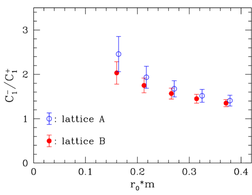
Figure 5: The fitted value of the ratio $C_{1}^{-}/C_{1}^{+}$ plotted versus the bare quark mass in units of $r_{0}$. The symbols are slightly displaced for clarity.

In Fig. 5 we plot the results for the asymptotic value of $C_{1}^{-}/C_{1}^{+}$ for both our lattices as a function of the bare quark mass in units of the hadronic radius $r_{0}$ [?]. At the smallest quark mass the ratio of correlators of operators transforming under irreducible representations of dimensions 20 and 84 is clearly greater than one. Furthermore, one observes a clear trend for this ratio to increase as the chiral limit is approached.

At leading order in ChPT the connection between $C_{1}^{-}/C_{1}^{+}$ and the ratio $g_{1}^{-}/g_{1}^{+}$ of LECs is given by

$$\frac{g_{1}^{-}}{g_{1}^{+}}=\frac{k_{1}^{-}}{k_{1}^{+}}\left.\frac{C_{1}^{-}(x_{0},y_{0})}{C_{1}^{+}(x_{0},y_{0})}\right|_{\rm ren},$$ (7.92)

where the subscript “ren” reminds us that the four-quark operators in the lattice-regularised theory must be related to a particular continuum scheme. Thus, in order to estimate $g_{1}^{-}/g_{1}^{+}$ it suffices to multiply $C_{1}^{-}/C_{1}^{+}$ by the relevant short-distance factors. When interpreted in this way, our results indicate a significant enhancement of the $\Delta{I}=1/2$ amplitude from long-distance QCD effects alone. However, the prediction of leading-order ChPT in eq. (7.92) implies that there should be no significant mass dependence in the ratio, a behaviour which is not reflected in our results.

Clearly, NLO effects must be taken into account. In the $p$-regime they depend on many unknown effective couplings, while, as we have shown in this paper, they can be computed in the $\epsilon$-regime without adding any extra parameters (see eqs. (5.53) and (5.52)). Since we lack any data in the $\epsilon$-regime, the NLO matching of $C_{1}^{-}/C_{1}^{+}$ to $g_{1}^{-}/g_{1}^{+}$ cannot be performed here. However, in order to illustrate how the NLO formulae might be used, we note that for lattice B the correction factor $H(x_{0},y_{0})$ evaluates to 2.262, independent of $x_{0}$ and $y_{0}$. Thus, if long-distance QCD effects alone were to enhance $g_{1}^{-}/g_{1}^{+}$ significantly, say, by a factor 2, then the ratio $C_{1}^{-}/C_{1}^{+}$ would have to be as large as $4-5$ in the $\epsilon$-regime.

We note, though, that the geometrical factor $\rho\equiv T/L$ enters $H(x_{0},y_{0})$, such that for space-time geometries with $T\gg L$ the NLO corrections can become large. For instance, on lattice B we have $\rho=2.5$, and one might expect that higher orders in the $\epsilon$-expansion cannot be neglected in this case (cf. Figs. 1 and 2).

Therefore, while we observe a good numerical signal for the ratio $C_{1}^{-}/C_{1}^{+}$, a quantitative interpretation of our results is not yet possible, since our masses are not in a regime where computable NLO corrections can be applied. Future simulations should therefore concentrate on the determination of $C_{1}^{-}/C_{1}^{+}$ for smaller quark masses. Moreover, choosing a small value of $T/L$, while keeping the spatial box length reasonably large (e.g. $L\;\raisebox{-2.58334pt}{$\stackrel{{\scriptstyle\textstyle{>}}}{{\sim}}$}\;1.5\,{\rm fm}$) will lead to better convergence properties of ChPT in the $\epsilon$-regime.

8 Summary and conclusions

We have outlined a computational strategy which allows to disentangle and quantify several possible origins of the $\Delta{I}=1/2$ rule using lattice simulations of QCD. The main idea is to consider the $\Delta{S}=1$ weak interactions with an active charm quark and to compute correlation functions for $K\to\pi$ transitions, whose values are subsequently matched to the LECs which parameterise the weak Hamiltonian in the effective low-energy theory. While the mass-degenerate case, $m_{u}=m_{d}=m_{s}=m_{c}$, allows to quantify contributions to the $\Delta{I}=1/2$ enhancement from long-distance effects that are not due to a large charm quark mass, the effects of physics at scales around $m_{c}$ can be estimated by increasing $m_{c}$ above $m_{u}$ and evaluating the “Eye”-diagram in addition to the “Figure-8”-graph. From the behaviour of the ratio of amplitudes as a function of $m_{c}$ one will be able to infer whether QCD long-distance effects are merely amplified by the splitting between up and charm quark masses, or whether the $\Delta{I}=1/2$ rule is due to modes at a specific energy scale, which should manifest itself as a sharp change in magnitude.

A key ingredient in our strategy is the use of fermionic discretisations which preserve chiral symmetry at non-zero lattice spacing (Ginsparg-Wilson fermions). In this case the renormalisation patterns of the relevant dimension-6 operators which are found in the continuum carry over to the lattice theory without modification. Moreover, the matching to the expressions of ChPT can be performed in a conceptually clean manner. Furthermore, the $\epsilon$-regime of ChPT offers a firm theoretical framework for the determination of LECs: owing to the specific chiral counting rules of the $\epsilon$-expansion, no additional interaction terms are generated in the effective weak part at NLO. By contrast, for the conventional chiral expansion ($p$-expansion) the matching to QCD at NLO involves coupling terms whose coefficients are unknown.

Our studies have revealed, though, that fairly large volumes are required in order to guarantee reliable results. The slow convergence of ChPT in the $\epsilon$-regime is indicated in Figs. 1 and 2, which demonstrate that corrections are relatively small only for $L\;\raisebox{-2.58334pt}{$\stackrel{{\scriptstyle\textstyle{>}}}{{\sim}}$}\;2.0\,{\rm fm}$. The use of asymmetric lattices slows down the convergence further. Since lattice simulations are typically performed with $T>L$, in order to be able to isolate the asymptotic behaviour of Euclidean correlation functions, whilst keeping the total number of lattice sites at a manageable level, this may render future numerical simulations relatively expensive.

We have performed numerical simulations in the SU(4)-symmetric case in the quenched approximation, with masses corresponding to the $p$-regime. The results show that the matching of $C_{1}^{-}/C_{1}^{+}$ to $g_{1}^{-}/g_{1}^{+}$ at leading order is clearly insufficient. On the other hand, for the reasons explained above, adjusting the kinematical variables so that NLO matching can be performed reliably in the $\epsilon$-regime is numerically expensive. In fact, the computational cost of simulating the kinematical regime where the $p$-expansion at leading order is valid might be even of comparable size. Which of these alternatives is to be preferred must be decided by future simulations.

We have also investigated the effects of a heavier charm quark in ChPT. These studies have shown that there is indeed a larger contribution to $\Delta{I}=1/2$ transitions when the charm quark mass is increased above the masses of the $u,\,d$ and $s$ quarks but kept below the chiral scale $\Lambda_{\chi}$. Since only moderately heavy charm quark masses can be studied safely in ChPT, numerical simulations must be performed to confirm this result. This will be the subject of our future simulations, in which we will evaluate the necessary “Eye”-diagrams. Furthermore, we intend to improve on the systematics of our earlier runs, by using lattices with smaller $T/L$ and going closer to the chiral limit.

Acknowledgements

We are indebted to Martin Lüscher, whose participation in the early stages of this project was instrumental to our study. We would like to thank him for many illuminating discussions and a careful reading of the manuscript. We are also grateful to Christian Hoelbling, Karl Jansen and Laurent Lellouch for interesting discussions. Our simulations were performed on PC clusters at DESY Hamburg, the Leibniz-Rechenzentrum der Bayerischen Akademie der Wissenschaften, the Max-Planck-Institut für Plasmaphysik in Garching and at the University of Valencia. We wish to thank all these institutions for support and the staff of their computer centers for technical help. L.G. acknowledges partial support by the EU under contract HPRN-CT-2002-00311 (EURIDICE). P.H. was supported by the CICYT (Project No. FPA2002-00162) and by the Generalitat Valenciana (Project No. CTIDIA/2002/5).

Appendix A Four-quark representations

In this appendix, we provide for completeness some aspects of the SU(4) classification of four-quark operators. For further details see, for instance, the complete presentation in [?]. We consider an operator $O_{\alpha\beta\gamma\delta}$ which transforms under the $\bf 4^{*}\otimes 4^{*}\otimes 4\otimes 4$ representation of SU(4) and decompose it into its irreducible parts. To this end we define the projected operators

$$O_{\alpha\beta\gamma\delta}^{\sigma}\equiv(P_{1}^{\sigma})_{\alpha\beta\gamma\delta;\lambda\nu\rho\tau}O_{\lambda\nu\rho\tau},$$ (A.93)

$$\widehat{O}_{\alpha\beta\gamma\delta}^{\sigma}\equiv(P_{2}^{\sigma})_{\alpha\beta\gamma\delta;\lambda\nu\rho\tau}O_{\lambda\nu\rho\tau}^{\sigma},$$ (A.94)

where $\sigma=\pm 1$. The projectors $P_{1}^{\sigma},P_{2}^{\sigma}$ are given by

$$(P_{1}^{\sigma})_{\alpha\beta\gamma\delta;\lambda\nu\rho\tau} \equiv {\textstyle\frac{1}{4}}(\delta_{\alpha\lambda}\delta_{\beta\nu}+\sigma\delta_{\alpha\nu}\delta_{\beta\lambda})(\delta_{\gamma\rho}\delta_{\delta\tau}+\sigma\delta_{\gamma\tau}\delta_{\delta\rho}),$$ (A.95)

$$(P_{2}^{\sigma})_{\alpha\beta\gamma\delta;\lambda\nu\rho\tau} \equiv \delta_{\alpha\lambda}\delta_{\beta\nu}\delta_{\gamma\rho}\delta_{\delta\tau}+\frac{1}{(4+2\sigma)(4+\sigma)}(\delta_{\alpha\gamma}\delta_{\beta\delta}+\sigma\delta_{\alpha\delta}\delta_{\beta\gamma})\delta_{\lambda\rho}\delta_{\nu\tau}\phantom{\frac{1}{4+2\sigma}}$$

$$-\frac{1}{4+2\sigma}(\delta_{\alpha\gamma}\delta_{\beta\nu}\delta_{\delta\tau}\delta_{\lambda\rho}+\delta_{\beta\delta}\delta_{\alpha\lambda}\delta_{\gamma\rho}\delta_{\nu\tau}+\sigma\delta_{\alpha\delta}\delta_{\beta\nu}\delta_{\gamma\tau}\delta_{\lambda\rho}+\sigma\delta_{\beta\gamma}\delta_{\alpha\lambda}\delta_{\delta\rho}\delta_{\nu\tau}).$$ (A.96)

Furthermore we define

$$S^{\sigma}=O_{\kappa\lambda\kappa\lambda}^{\sigma},$$ (A.97)

$$R^{\sigma}_{\alpha\gamma}=O_{\alpha\lambda\gamma\lambda}^{\sigma}-{\textstyle\frac{1}{4}}\delta_{\alpha\gamma}S^{\sigma}.$$ (A.98)

Any four-quark operator $O_{\alpha\beta\gamma\delta}$ can then be decomposed into irreducible representations according to

$$O_{\alpha\beta\gamma\delta} = \sum_{\sigma=\pm}\left\{\widehat{O}_{\alpha\beta\gamma\delta}^{\sigma}+\frac{1}{4(4+\sigma)}(\delta_{\alpha\gamma}\delta_{\beta\delta}+\sigma\delta_{\alpha\delta}\delta_{\beta\gamma})S^{\sigma}\right.$$ (A.99)

$$\phantom{\sum_{\sigma=\pm}\Big{\{}\widehat{O}_{\alpha\beta\gamma\delta}^{\sigma}}\left.+\frac{1}{4+2\sigma}(\delta_{\alpha\gamma}R^{\sigma}_{\beta\delta}+\delta_{\beta\delta}R^{\sigma}_{\alpha\gamma}+\sigma\delta_{\alpha\delta}R^{\sigma}_{\beta\gamma}+\sigma\delta_{\beta\gamma}R^{\sigma}_{\alpha\delta})\right\}.\phantom{\alpha}$$

The operators $\widehat{O}_{\alpha\beta\gamma\delta}^{\pm}$, $R^{\pm}_{\alpha\gamma}$ and $S^{\pm}$ transform according to representations of the following dimensions:

$$\begin{array}[]{lcr lcr}\widehat{O}_{\alpha\beta\gamma\delta}^{+}&\hbox{:}&{\bf 84},&\quad\qquad R^{\pm}_{\alpha\gamma}&\hbox{:}&{\bf 15},\\ \widehat{O}_{\alpha\beta\gamma\delta}^{-}&\hbox{:}&{\bf 20},&\quad\qquad S^{\pm}&\hbox{:}&{\bf 1}.\end{array}$$ (A.100)

In eq. (2.9), the operators ${\cal Q}_{1}^{\pm}$ have been defined for the relevant physical flavour assignments. Their relations to the projected operators $\widehat{O}_{1}^{\pm}$ are given by

$${\cal Q}_{1}^{\pm}=2([\widehat{O}_{1}^{\pm}]_{suud}-[\widehat{O}_{1}^{\pm}]_{sccd}),$$ (A.101)

where $\widehat{O}_{1}^{\pm}$ are obtained from the generic four-quark operator $[O_{1}]_{\alpha\beta\gamma\delta}$ via eqs. (A.93) and (A.94).

Appendix B Exact chiral symmetry and CP

In this appendix we report the argument spelled out in [?], which shows that in lattice QCD with Ginsparg-Wilson fermions, the CP symmetry remains a useful tool in the analysis of operator mixing, if a chiral operator basis is chosen. Assuming that $D$ satisfies the Ginsparg-Wilson relation, we note that the quark action

$$S_{\rm F}=a^{4}\sum_{x}\left\{\overline{\psi}(x)[D\psi](x)+\overline{\psi}(x)\big{(}MP_{+}+M^{\dagger}P_{-}\big{)}\big{[}\big{(}1-{\textstyle\frac{1}{2}}{\bar{a}}D\big{)}\psi\big{]}(x)\right\}$$ (B.102)

is invariant under the exact $\rm SU(4)_{L}\times SU(4)_{R}$ symmetry group, provided the quark mass matrix $M$ is transformed according to the $\bf 4\otimes 4^{*}$ representation. If the mass matrix $M$ is chosen real and diagonal, the action is also invariant under parity and charge conjugation. The restriction to this case is not important, since chiral transformations can always be used to diagonalise $M$. However, four-quark operators such as

$${O}^{\pm}_{\alpha\beta\gamma\delta}=\big{(}\overline{\psi}_{\alpha}\gamma_{\mu}P_{-}\widetilde{\psi}_{\gamma}\big{)}\big{(}\overline{\psi}_{\beta}\gamma_{\mu}P_{-}\widetilde{\psi}_{\delta}\big{)}\pm(\gamma\leftrightarrow\delta)$$ (B.103)

do not transform in a simple way under CP. At the level of correlation functions of local fields, this is not a problem, because one can substitute

$$\widetilde{\psi}(x)=\big{(}1-{\textstyle\frac{1}{2}}{\bar{a}}M\big{)}^{-1}\left\{\psi(x)-{\textstyle\frac{1}{2}}{\bar{a}}\frac{{\delta}S_{\rm F}}{\delta\overline{\psi}(x)}\right\}$$ (B.104)

and perform a partial integration in the functional integral to eliminate the second term on the right-hand side. One then obtains the same correlation functions up to contact terms, but with the modified field $\widetilde{\psi}$ replaced by $(1-{\textstyle\frac{1}{2}}{\bar{a}}M)^{-1}\psi$.

In the case of the operators ${O}^{\pm}_{\alpha\beta\gamma\delta}$ one can show that all contact terms vanish after contracting the Dirac indices. When inserted in correlation functions of local fields at non-zero distances, one obtains the operator identity

$${O}^{\pm}_{\alpha\beta\gamma\delta} = \big{(}1-{\textstyle\frac{1}{2}}{\bar{a}}m_{\gamma}\big{)}^{-1}\big{(}1-{\textstyle\frac{1}{2}}{\bar{a}}m_{\delta}\big{)}^{-1}$$ (B.105)

$$\times\Big{\{}\big{(}\overline{\psi}_{\alpha}\gamma_{\mu}P_{-}\psi_{\gamma}\big{)}\big{(}\overline{\psi}_{\beta}\gamma_{\mu}P_{-}\psi_{\delta}\big{)}\pm(\gamma\leftrightarrow\delta)\Big{\}}.$$

Applying a CP transformation yields

$${O}^{\pm}_{\alpha\beta\gamma\delta}(x)\stackrel{{\scriptstyle\hbox{CP}}}{{\longrightarrow}}\frac{(1-{\textstyle\frac{1}{2}}{\bar{a}}m_{\alpha})(1-{\textstyle\frac{1}{2}}{\bar{a}}m_{\beta})}{(1-{\textstyle\frac{1}{2}}{\bar{a}}m_{\gamma})(1-{\textstyle\frac{1}{2}}{\bar{a}}m_{\delta})}\,{O}^{\pm}_{\gamma\delta\alpha\beta}(\tilde{x}),$$ (B.106)

where $\tilde{x}=(x_{0},-x_{1},-x_{2},-x_{3})$, and it is understood that the rule only applies in local correlation functions. The argumentation in the case of two-quark operators proceeds along exactly the same lines.

Appendix C Perturbative results for the anomalous dimensions $\gamma^{\sigma}(g)$

For convenience we recall that the RG $\beta$-function has a perturbative expansion

$$\beta(g)=-g^{3}\sum_{k=0}^{\infty}b_{k}g^{2k}\,,$$ (C.107)

with the universal one– and two–loop coefficients:

$$b_{0} = \frac{1}{(4\pi)^{2}}\left(\frac{11}{3}N_{\rm c}-\frac{2}{3}N_{\rm f}\right)\,,$$ (C.108)

$$b_{1} = \frac{1}{(4\pi)^{4}}\left(\frac{34}{3}N_{\rm c}^{2}-N_{\rm f}\left\{\frac{13}{3}N_{\rm c}-\frac{1}{N_{\rm c}}\right\}\right)\,.$$ (C.109)

The anomalous dimension of ${\cal{Q}}_{1}^{\sigma}$ has a perturbative expansion of the form

$$\gamma^{\sigma}(g)=g^{2}\sum_{k=0}^{\infty}\gamma^{\sigma}_{k}g^{2k}.$$ (C.110)

The one–loop coefficients $\gamma^{\sigma}_{0}$ were first obtained by Gaillard and Lee [?],

$$\gamma^{\sigma}_{0}=-\frac{1}{(4\pi)^{2}}\frac{6\sigma(N_{\rm c}-\sigma)}{N_{\rm c}}\,.$$ (C.111)

The two–loop coefficients depend on the scheme and on the way $\gamma_{5}$ is handled. The first such two–loop computation was performed by Altarelli, Curci, Martinelli and Petrarca [?] using dimensional reduction [?]. The computation in the HV(MS) scheme was carried out much later with the result [?]:

$$\gamma^{\sigma}_{1}=\frac{1}{(4\pi)^{4}}\frac{(N_{\rm c}-\sigma)}{2N_{\rm c}}\left[-\frac{88}{3}N_{\rm c}^{2}+21+\frac{16}{3}N_{\rm c}N_{\rm f}-\sigma\left\{\frac{157}{3}N_{\rm c}+\frac{57}{N_{\rm c}}-\frac{28}{3}N_{\rm f}\right\}\right]\,.$$ (C.112)

Denoting the operators in the HV scheme by $({\cal{Q}}_{1}^{\sigma})_{\rm HV}$, the renormalised operators of any other satisfactory scheme S should be related to these merely by a finite multiplicative renormalisation,

$$({\cal{Q}}_{1}^{\sigma})_{\rm S}={\cal X}^{\sigma}_{\rm S}(g)({\cal{Q}}_{1}^{\sigma})_{\rm HV}\,.$$ (C.113)

Assuming that the normalisations are such that ${\cal X}^{\sigma}_{\rm S}=1$ at tree level, the coefficients have a perturbative expansion of the form

$${\cal X}^{\sigma}_{\rm S}(g)=1+\sum_{k=1}^{\infty}x^{\sigma}_{\rm S;k}g^{2k}\,.$$ (C.114)

The one-loop coefficients have been computed in various schemes, e.g. in the RI scheme one has

$$x^{\sigma}_{\rm RI;1}=-\frac{1}{(4\pi)^{2}}\frac{(N_{\rm c}-\sigma)}{2N_{\rm c}}\left[4N_{\rm c}-6\sigma\left\{1-4\ln(2)\right\}\right]\,.$$ (C.115)

For Ginsparg-Wilson fermions, as defined in Sect. 3, one has

$$x^{\sigma}_{\rm GW;1}=\frac{1}{(4\pi)^{2}}\frac{(N_{\rm c}-\sigma)}{2N_{\rm c}}\left[X_{0}\sigma+X_{1}N_{\rm c}\right]\,,$$ (C.116)

with

$$X_{0} = 4B_{\rm V}-2B_{\rm S}+2B_{\psi}+6\,,$$ (C.117)

$$X_{1} = 2B_{\rm V}+2B_{\psi}-4\,,$$ (C.118)

where the functions $B_{\rm V},B_{\rm S},B_{\psi}$ depend on the parameter $s$, and some numerical values can be found in Table 1 of ref. [?]. Corresponding values for the $X_{i}$ are given in Table 3.

The anomalous dimensions of the operators in scheme S are related to those in the HV scheme by

$$\gamma^{\sigma}_{\rm S}=\gamma^{\sigma}+\beta(g)\frac{\partial}{\partial g}\ln{\cal X}^{\sigma}_{\rm S}(g)\,.$$ (C.119)

Denoting the coefficients in the perturbative expansion of $\gamma^{\sigma}_{\rm S}$ in the ${\rm\overline{MS\kern-0.50003pt}\kern 0.50003pt}$ coupling (as in Eq. (C.110)) by $\gamma^{\sigma}_{\rm S;k}$, the lowest order coefficients are given by

$$\gamma^{\sigma}_{\rm S;0} = \gamma^{\sigma}_{0}\,,$$ (C.120)

$$\gamma^{\sigma}_{\rm S;1} = \gamma^{\sigma}_{1}-2b_{0}x^{\sigma}_{\rm S;1}\,.$$ (C.121)

For completeness we mention that for the lattice computations it is often convenient to write the expressions in Sect. 4 in terms of lattice couplings. In this case, as an intermediate step, it is useful to know the relation of the ${\rm\overline{MS\kern-0.50003pt}\kern 0.50003pt}$ coupling to the bare lattice coupling:

$${g}^{2}_{{\rm\overline{MS\kern-0.35002pt}\kern 0.35002pt}}(ta^{-1})=g_{0}^{2}+\frac{d_{1}(t)}{4\pi}g_{0}^{4}+\dots\,.$$ (C.122)

To obtain the anomalous dimensions expressed in terms of the lattice coupling to two-loop level, it is sufficient to know the coefficient $d_{1}$ which takes the form:

$$d_{1}(t)=-8\pi b_{0}\ln(t)+d_{10}+d_{11}N_{\rm f}\,.$$ (C.123)

The term $d_{10}$ depends on the pure gauge action; e.g. for the Wilson gauge action it was computed long ago by A. and P. Hasenfratz [?] and is given by

$$d_{10} = -\frac{\pi}{2N_{\rm c}}+k_{1}N_{\rm c}\,,$$ (C.124)

$$k_{1} = 2.135730074078457(2)\,.$$ (C.125)

The term $d_{11}$ in (C.123) for GW fermions depends on the parameter $s$ and is given by

$$d_{11}(s)=4\pi\left[\frac{5}{72\pi^{2}}+d_{1,1}(\rho)+d_{1,2}(\rho)\right]\,,$$ (C.126)

where numerical values for the functions $d_{1,i}(\rho),i=1,2$, with $\rho=1+s$, are given in Table 1 of ref. [?]. Corresponding values for $d_{11}(s)$ are given in Table 3.

$s\,\,\,$	$X_{0}\,\,\,\,\,\,$	$X_{1}\,\,\,\,\,\,$	$d_{11}$
$-0.8$	$-462.169$	$-472.573$	$0.287181$
$-0.7$	$-292.939$	$-302.192$	$0.256186$
$-0.6$	$-209.059$	$-217.347$	$0.235334$
$-0.5$	$-159.227$	$-166.669$	$0.219891$
$-0.4$	$-126.366$	$-133.048$	$0.207873$
$-0.3$	$-103.174$	$-109.157$	$0.198305$
$-0.2$	$-86.004$	$-91.337$	$0.190679$
$-0.1$	$-72.836$	$-77.557$	$0.184743$
$\phantom{-}0.0$	$-62.460$	$-66.599$	$0.180413$
$\phantom{-}0.1$	$-54.108$	$-57.689$	$0.177735$
$\phantom{-}0.2$	$-47.270$	$-50.313$	$0.176883$
$\phantom{-}0.3$	$-41.593$	$-44.113$	$0.178175$
$\phantom{-}0.4$	$-36.827$	$-38.836$	$0.182126$
$\phantom{-}0.5$	$-32.787$	$-34.295$	$0.189537$
$\phantom{-}0.6$	$-29.338$	$-30.351$	$0.201685$
$\phantom{-}0.7$	$-26.376$	$-26.896$	$0.220694$
$\phantom{-}0.8$	$-23.820$	$-23.848$	$0.250421$

Table 3: Values of functions $X_{i}$ appearing in eq. (C.116), and $d_{11}(s)$ appearing in eq. (C.123).

Appendix D Correlators in Chiral Perturbation Theory

In this appendix we describe the calculation of correlation functions of left-handed charges and operators $\widehat{\cal O}_{1}^{\sigma}$ for a finite periodic box with volume $V=T\cdot{L_{1}}\cdot{L_{2}}\cdot{L_{3}}$, at order $\epsilon^{2}$ in ChPT. The same calculation in the SU(3)-symmetric case has already been published in ref. [?], which can be consulted for further details. In particular, we note that the sets of diagrams which appear at this order in the $\epsilon$-expansion, are identical to the SU(4)-case considered here, and are depicted in Figs. 1 and 3 of [?].

The result for the correlation function ${\cal C}^{ab}$ at order $\epsilon^{2}$ is

$${\cal C}^{ab} = {\rm Tr}(T^{a}T^{b})\frac{F^{2}}{2T}\bigg{\{}1+\frac{N_{\rm f}}{F^{2}}\bigg{[}\frac{\beta_{1}}{V^{1/2}}-\frac{T^{2}k_{00}}{V}\bigg{]}$$ (D.127)

$$+\frac{2\Sigma T^{2}}{N_{\rm f}F^{2}}\left\langle{\rm Re}\,{\rm Tr}[MU_{0}{\rm e}^{i\theta/N_{\rm f}}]\right\rangle_{\theta,U_{0}}h_{1}\Big{(}\frac{x_{0}}{T}\Big{)}\bigg{\}},$$

where $N_{\rm f}=4$, and the function $h_{1}$ is given by [?]

$$h_{1}(\tau)={\textstyle\frac{1}{2}}\Big{[}\big{(}|\tau|-{\textstyle\frac{1}{2}}\big{)}^{2}-{\textstyle\frac{1}{12}}\Big{]}.$$ (D.128)

The definitions of the coefficients $\beta_{1}$ and $k_{00}$, which depend on the geometry of the box, can be found in [?]. Examples of numerical values are listed in Table 4.

$T/L$	$\beta_{1}$		$k_{00}$
32/32	0.	14046	$0.07023=\beta_{1}/2$
32/28	0.	13872	0.07826
32/24	0.	13215	0.08186
32/20	0.	11689	0.08307
32/16	0.	08360	0.08331
32/12	0.	00582	0.08333
32/8	$-0$.	21510	0.08333

Table 4: Some numerical values for $\beta_{1}$ and $k_{00}$, for geometries with $L_{1}=L_{2}=L_{3}\equiv{L}$.

For $[\widehat{\cal C}_{1}^{\pm}(x_{0},y_{0})]^{ab}_{\alpha\beta\gamma\delta}$ the general expression reads

$$[\widehat{\cal C}_{1}^{\pm}(x_{0},y_{0})]^{ab}_{\alpha\beta\gamma\delta} = \hat{\Delta}^{ab,\sigma}_{\alpha\beta\gamma\delta}\frac{F^{4}}{4T^{2}}\bigg{\{}1+(N_{\rm f}+\sigma)\frac{2}{F^{2}}\bigg{[}\frac{\beta_{1}}{V^{1/2}}-\frac{T^{2}k_{00}}{V}\bigg{]}$$ (D.129)

$$+\frac{2\Sigma T^{2}}{N_{\rm f}F^{2}}\left\langle{\rm Re}\,{\rm Tr}[MU_{0}{\rm e}^{i\theta/N_{\rm f}}]\right\rangle_{\theta,U_{0}}\bigg{[}h_{1}\Big{(}\frac{x_{0}}{T}\Big{)}+h_{1}\Big{(}\frac{y_{0}}{T}\Big{)}\bigg{]}\bigg{\}}.$$

Contact terms have been dropped in this expression, and we may assume that $x_{0},\,y_{0}$ are on opposite sides relative to the origin, i.e. $x_{0}<0,y_{0}>0$. The flavour structure is encoded in the tensor

$$\hat{\Delta}^{ab,\sigma}_{\alpha\beta\gamma\delta} \equiv {\textstyle\frac{1}{2}}\Big{(}T_{\gamma\alpha}^{\{a}T_{\delta\beta}^{b\}}+\sigma T_{\gamma\beta}^{\{a}T_{\delta\alpha}^{b\}}\Big{)}+\frac{1}{(4+\sigma)(4+2\sigma)}\Big{(}\delta_{\gamma\beta}\delta_{\delta\alpha}+\sigma\delta_{\gamma\alpha}\delta_{\delta\beta}\Big{)}{\rm Tr}(T^{a}T^{b})$$ (D.130)

$$-\frac{1}{2(4+2\sigma)}\Big{(}\delta_{\gamma\beta}\{T^{a},T^{b}\}_{\delta\alpha}+\delta_{\delta\alpha}\{T^{a},T^{b}\}_{\gamma\beta}$$

$$\phantom{-\frac{1}{2(4+2\sigma)}}+\sigma\delta_{\gamma\alpha}\{T^{a},T^{b}\}_{\delta\beta}+\sigma\delta_{\delta\beta}\{T^{a},T^{b}\}_{\gamma\alpha}\Big{)},$$

where

$$T_{\gamma\alpha}^{\{a}T_{\delta\beta}^{b\}}\equiv T^{a}_{\gamma\alpha}T^{b}_{\delta\beta}+T^{a}_{\delta\beta}T^{b}_{\gamma\alpha}.$$ (D.131)

In order to study the case of a light charm quark, one can choose a diagonal, degenerate mass matrix and generators such that

$$T^{a}_{\tau\omega}=\delta_{\tau\gamma}\delta_{\omega\alpha},\qquad T^{b}_{\tau\omega}=\delta_{\tau\delta}\delta_{\omega\beta},$$ (D.132)

where $\alpha,\beta,\gamma,\delta$ are assumed all fixed and different. In this case one finds that $\hat{\Delta}^{ab}=1/2$, and for a symmetric spatial volume and vanishing vacuum angle $\theta$ one recovers the expressions in eqs. (5.46) and (5.3).

Correlation functions in sectors of fixed topology, characterised by an index $\nu$, can be obtained from those for fixed vacuum angle $\theta$ via Fourier transform. If we assume a diagonal mass matrix and define

$$Z_{\theta}(u/2)=\int_{U_{0}}{\rm e}^{(u/2){\rm Re}\,{\rm Tr}[U_{0}\exp(i\theta/N_{\rm f})]},\quad Z_{\nu}(u/2)=\frac{1}{2\pi}\int_{0}^{2\pi}{\rm d}\theta\,{\rm e}^{-i\nu\theta}Z_{\theta}(u/2),$$ (D.133)

the quantity $C_{\theta}(u/2)$ in eqs. (5.46) and (5.3) gets simply replaced by

$$C_{\theta}(u/2)\equiv\frac{2}{N_{\rm f}}\frac{\partial}{\partial u}\ln Z_{\theta}(u/2)\longrightarrow\frac{2}{N_{\rm f}}\frac{\partial}{\partial u}\ln Z_{\nu}(u/2)\equiv C_{\nu}(u/2).$$ (D.134)

In the small and large mass regions, $C_{\nu}(u/2)$ is approximately given by

$$C_{\nu}(u/2)\approx\left\{\begin{array}[]{cl}2|\nu|/u,&u\ll 1,\\ 1,&u\gg 1.\end{array}\right.$$ (D.135)

References

- [1] M.K. Gaillard and B.W. Lee, Phys. Rev. Lett. 33 (1974) 108; G. Altarelli and L. Maiani, Phys. Lett. B52 (1974) 351
- [2] N. Cabibbo, G. Martinelli and R. Petronzio, Nucl. Phys. B244 (1984) 381; R.C. Brower, G. Maturana, M.B. Gavela and R. Gupta, Phys. Rev. Lett. 53 (1984) 1318
- [3] C.W. Bernard, T. Draper, A. Soni, H.D. Politzer and M.B. Wise, Phys. Rev. D32 (1985) 2343
- [4] L. Maiani and M. Testa, Phys. Lett. B245 (1990) 585
- [5] M. Bochicchio, L. Maiani, G. Martinelli, G.C. Rossi and M. Testa, Nucl. Phys. B262 (1985) 331; L. Maiani, G. Martinelli, G.C. Rossi and M. Testa, Nucl. Phys. B289 (1987) 505
- [6] C. Pena, S. Sint and A. Vladikas, JHEP 0409 (2004) 069
- [7] R. Frezzotti and G.C. Rossi, JHEP 0410 (2004) 070
- [8] L. Lellouch and M. Lüscher, Commun. Math. Phys. 219 (2001) 31
- [9] C.J.D. Lin, G. Martinelli, C.T. Sachrajda and M. Testa, Nucl. Phys. B619 (2001) 467
- [10] P.H. Ginsparg and K.G. Wilson, Phys. Rev. D25 (1982) 2649
- [11] D.B. Kaplan, Phys. Lett. B288 (1992) 342; Nucl. Phys. B (Proc. Suppl.) 30 (1993) 597
- [12] Y. Shamir, Nucl. Phys. B406 (1993) 90
- [13] V. Furman and Y. Shamir, Nucl. Phys. B439 (1995) 54
- [14] P. Hasenfratz, Nucl. Phys. B (Proc. Suppl.) 63 (1998) 53; Nucl. Phys. B525 (1998) 401
- [15] P. Hasenfratz, V. Laliena and F. Niedermayer, Phys. Lett. B427 (1998) 125
- [16] H. Neuberger, Phys. Lett. B417 (1998) 141; ibid. B427 (1998) 353
- [17] M. Lüscher, Phys. Lett. B428 (1998) 342
- [18] P. Hernández, K. Jansen and M. Lüscher, Nucl. Phys. B552 (1999) 363
- [19] S. Capitani and L. Giusti, Phys. Rev. D64 (2001) 014506
- [20] CP-PACS Collaboration (J.I. Noaki et al.), Phys. Rev. D68 (2003) 014501
- [21] RBC Collaboration, (T. Blum et al.), Phys. Rev. D68 (2003) 114506
- [22] M.A. Shifman, A.I. Vainshtein and V.I. Zakharov, Nucl. Phys. B120 (1977) 316
- [23] W. A. Bardeen, A. J. Buras and J. M. Gerard, Phys. Lett. B192 (1987) 138
- [24] J. Kambor, J. Missimer and D. Wyler, Nucl. Phys. B346 (1990) 17; Phys. Lett. B261 (1991) 496
- [25] M. Neubert and B. Stech, Phys. Rev. D44 (1991) 775
- [26] A. Pich and E. de Rafael, Nucl. Phys. B358 (1991) 311; M. Jamin and A. Pich, Nucl. Phys. B425 (1994) 15
- [27] V. Antonelli, S. Bertolini, M. Fabbrichesi and E. I. Lashin, Nucl. Phys. B469 (1996) 181; S. Bertolini, J. O. Eeg, M. Fabbrichesi and E. I. Lashin, Nucl. Phys. B514 (1998) 63
- [28] H. Georgi, Weak Interactions and Modern Particle Theory (Benjamin/Cummings, Menlo Park, California, 1984)
- [29] M. Lüscher, Irreducible representations of SU(4), unpublished notes (2002)
- [30] L. Giusti and M. Lüscher, Mixing of the weak interaction hamiltonian, unpublished notes (2002)
- [31] M. Lüscher, Four-quark operators in QCD, unpublished notes (2002)
- [32] P. Hasenfratz, Nucl. Phys. B (Proc. Suppl.) 106 (2002) 159
- [33] G. Altarelli, G. Curci, G. Martinelli and S. Petrarca, Nucl. Phys. B187 (1981) 461
- [34] A.J. Buras and P.H. Weisz, Nucl. Phys. B333 (1990) 66
- [35] M. Ciuchini, E. Franco, V. Lubicz, G. Martinelli, I. Scimemi and L. Silvestrini, Nucl. Phys. B523 (1998) 501
- [36] A.J. Buras, M. Misiak and J. Urban, Nucl. Phys. B586 (2000) 397
- [37] ALPHA Collaboration (S. Capitani et al.), Nucl. Phys. B544 (1999) 669
- [38] S. Aoki and Y. Kuramashi, Phys. Rev. D63 (2001) 054504
- [39] S. Capitani and L. Giusti, Phys. Rev. D62 (2000) 114506
- [40] T. DeGrand, Phys. Rev. D67 (2003) 014507
- [41] N. Garron, L. Giusti, C. Hoelbling, L. Lellouch and C. Rebbi, Phys. Rev. Lett. 92 (2004) 042001
- [42] J. Gasser and H. Leutwyler, Phys. Lett. B188 (1987) 477; Nucl. Phys. B307 (1988) 763
- [43] H. Neuberger, Phys. Rev. Lett. 60 (1988) 889; Nucl. Phys. B300 (1988) 180
- [44] F.C. Hansen and H. Leutwyler, Nucl. Phys. B350 (1991) 201
- [45] P. Hernández and M. Laine, JHEP 0301 (2003) 063
- [46] P. Hernández, K. Jansen and L. Lellouch, Phys. Lett. B469 (1999) 198
- [47] T. DeGrand, Phys. Rev. D63 (2001) 034503
- [48] P. Hasenfratz, S. Hauswirth, T. Jörg, F. Niedermayer and K. Holland, Nucl. Phys. B643 (2002) 280
- [49] L. Giusti, P. Hernández, M. Laine, P. Weisz and H. Wittig, JHEP 0401 (2004) 003
- [50] L. Giusti, P. Hernández, M. Laine, P. Weisz and H. Wittig, JHEP 0404 (2004) 013
- [51] F.C. Hansen, Nucl. Phys. B345 (1990) 685
- [52] H. Leutwyler and A. Smilga, Phys. Rev. D46 (1992) 5607
- [53] L. Giusti, G.C. Rossi and M. Testa, Phys. Lett. B587 (2004) 157
- [54] M. Lüscher, Phys. Lett. B593 (2004) 296
- [55] P. Hasenfratz and H. Leutwyler, Nucl. Phys. B343 (1990) 241
- [56] C.W. Bernard and M.F.L. Golterman, Phys. Rev. D46 (1992) 853
- [57] S.R. Sharpe, Phys. Rev. D46 (1992) 3146
- [58] P.H. Damgaard and K. Splittorff, Phys. Rev. D62 (2000) 054509
- [59] P.H. Damgaard, M.C. Diamantini, P. Hernández and K. Jansen, Nucl. Phys. B629 (2002) 445
- [60] M. Golterman and E. Pallante, JHEP 0110 (2001) 037; Phys. Rev. D69 (2004) 074503
- [61] P.H. Damgaard, P. Hernández, K. Jansen, M. Laine and L. Lellouch, Nucl. Phys. B656 (2003) 226
- [62] P. Hernández and M. Laine, JHEP 0409 (2004) 018
- [63] J. Gasser and H. Leutwyler, Nucl. Phys. B250 (1985) 465
- [64] J. Bijnens, G. Ecker and J. Gasser, hep-ph/9411232
- [65] R.J. Crewther, Nucl. Phys. B264 (1986) 277
- [66] L. Giusti, Ch. Hoelbling, M. Lüscher and H. Wittig, Comput. Phys. Commun. 153 (2003) 31
- [67] W. Bietenholz, T. Chiarappa, K. Jansen, K.I. Nagai and S. Shcheredin, JHEP 0402 (2004) 023
- [68] L. Giusti, M. Lüscher, P. Weisz and H. Wittig, JHEP 0311 (2003) 023
- [69] T. DeGrand and S. Schaefer, Comput. Phys. Commun. 159 (2004) 185
- [70] R.G. Edwards, Nucl. Phys. B (Proc. Suppl.) 106 (2002) 38, and references therein
- [71] W. Siegel, Phys. Lett. B84 (1979) 193
- [72] A. Hasenfratz and P. Hasenfratz, Nucl. Phys. B193 (1981) 210
- [73] C. Alexandrou, H. Panagopoulos and E. Vicari, Nucl. Phys. B571 (2000) 257
- [74] R. Sommer, Nucl. Phys. B411 (1994) 839; ALPHA Collaboration (M. Guagnelli et al.), Nucl. Phys. B535 (1998) 389; S. Necco and R. Sommer, Nucl. Phys. B622 (2002) 328
- [75] SPQcdR Collaboration (P. Boucaud et al.), Nucl. Phys. B (Proc. Suppl.) 106 (2002) 329; J. Laiho and A. Soni, Phys. Rev. D 65 (2002) 114020; hep-lat/0306035; C.J.D. Lin, G. Martinelli, E. Pallante, C.T. Sachrajda and G. Villadoro, Nucl. Phys. B650 (2003) 301