Lattice Gauge Fixing as Quenching and the Violation of Spectral Positivity

Abstract

Lattice Landau gauge and other related lattice gauge fixing schemes are known to violate spectral positivity. The most direct sign of the violation is the rise of the effective mass as a function of distance. The origin of this phenomenon lies in the quenched character of the auxiliary field $g$ used to implement lattice gauge fixing, and is similar to quenched QCD in this respect. This is best studied using the PJLZ formalism, leading to a class of covariant gauges similar to the one-parameter class of covariant gauges commonly used in continuum gauge theories. Soluble models are used to illustrate the origin of the violation of spectral positivity. The phase diagram of the lattice theory, as a function of the gauge coupling $\beta$ and the gauge-fixing parameter $\alpha$, is similar to that of the unquenched theory, a Higgs model of a type first studied by Fradkin and Shenker. The gluon propagator is interpreted as yielding bound states in the confined phase, and a mixture of fundamental particles in the Higgs phase, but lattice simulation shows the two phases are connected. Gauge field propagators from the simulation of an $SU(2)$ lattice gauge theory on a $20^{4}$ lattice are well described by a quenched mass-mixing model. The mass of the lightest state, which we interpret as the gluon mass, appears to be independent of $\alpha$ for sufficiently large $\alpha$.

I Introduction

Although many interesting properties of a lattice gauge theory can be determined without gauge fixing, there are several reasons why it is needed. At a fundamental level, gauge fixing is necessary to make the connection between continuum and lattice gauge fields. Gauge fixing has also been a key technique in lattice studies of confinement as well Greensite:2003bk , and may help differentiate between different models of confinement. For example, continuum theories of the origin of confinement often make predictions about the gauge field propagator; see Ref. Mandula:nj for a review. Finally, gauge fixing may be needed to determine important properties of the quark-gluon plasma phase of QCD, such as screening masses, which are contained in the finite-temperature gluon propagator Heller:1995qc ; Heller:1997nq ; Cucchieri:2000cy ; Nakamura:2003pu .

Techniques for lattice gauge fixing have been known for some time Mandula:rh . It has been clear from the beginning that non-Abelian lattice gauge field propagators show a violation of spectral positivity. In a theory respecting spectral positivity, the Källén-Lehmann representation for a typical wall-to-wall two-point function has the form

$$G(t)=\int_{0}^{\infty}dm^{2}\,\,\rho\left(m^{2}\right)\frac{1}{2m}e^{-m\left|t\right|}$$ (1)

where $\rho$ is everywhere non-negative. Wall sources set all momenta transverse to the direction of propagation to zero. The effective mass defined by

$$m_{eff}\left(t\right)=-\frac{d}{dt}\ln G(t)$$ (2)

can be thought of as an average mass $\left\langle m(t)\right\rangle$, where the average is taken over $\rho\left(m^{2}\right)\exp({-m\left|t\right|})/{2m}.$ It follows that

$$\frac{d}{dt}m_{eff}\left(t\right)=\left\langle m(t)\right\rangle^{2}-\left\langle m^{2}(t)\right\rangle\leq 0.$$ (3)

The positivity of $\rho$ implies that the effective mass is a non-increasing function of $t$ which goes to the lightest mass propagated in the limit $t\rightarrow\infty$.

Gauge invariant operators which couple to glueball states show this behavior, but the gluon propagator does not. Covariant gauge gluon propagators have an effective mass increasing with distance. This is not too surprising: we know from perturbation theory that covariant gauges contain states of negative norm. However, that knowledge has neither explained the form of the lattice gluon propagator nor aided in the interpretation of the mass parameters measured from it. In fact, the particular form of spectral positivity violation observed for non-Abelian models is not observed in the $U(1)$ case Coddington:yz , which also has negative-norm states in covariant gauges.

In lattice simulations, gauge fixing has typically involved choosing a particular configuration on each gauge orbit. A brief review of this approach is given in Ref. Mandula:nj . In the continuum, on the other hand, gauge fixing most often includes a parameter that causes the functional integral to peak around a particular configuration on the gauge orbit. The PJLZ formalism, a comparable formalism for lattice gauge fixing, first appeared in Refs. Parrinello:1990pm ; Zwanziger:tn . The strong-coupling expansion was developed in Ref. Fachin:1991pu and the gluon propagator was studied in Ref. Henty:1996kv . This formalism was used in a discussion of Abelian projection in lattice theories Ogilvie:1998wu . There it was shown that Abelian projection without gauge fixing leads to an equality of the asymptotic string tensions in the underlying non-Abelian theory and the projected Abelian theory. Furthermore, the string tensions were proven to be equal with gauge fixing, provided the gauge fixing procedure respects spectral positivity. The failure of spectral positivity demonstrated in Ref. Aubin:2003ih explains the string tension discrepancies noted in lattice studies of Abelian projection. A lattice study of the phase structure of the projected theory as a function of the gauge-fixing parameter was carried out in Ref. Mitrjushkin:2001hr .

Our aim in this work is to demonstrate that spectral positivity is violated in lattice gauge fixing by mechanisms related to those encountered in quenched QCD. Specifically, we argue that the gluon propagator has a double pole structure similar to that of the $\eta^{\prime}$. We show in Sec. II that the PJLZ formalism makes clear that lattice gauge fixing is a form of quenching, with the gauge transformations acting as quenched fields. In Sec. III, we develop a general formalism for quenched fields, and apply that formalism to gauge fixing. We show that in the case of a $U(1)$ gauge theory, spectral positivity is maintained. Sec. IV examines two useful simple models for quenched fields based on mass mixing between a quenched and an unquenched field. The first model involves scalars; the second involves vector fields, and will be used to fit the results of our lattice simulations. In Sec. V, we discuss the phase diagram of the gauge-fixed model, using the interpretation of gauge fixing as a quenched Higgs model. As first discussed by Fradkin and Shenker, the nominal Higgs and confining phases of the unquenched model are connected, and this carries over to the quenched version. We propose interpretations for the lattice gauge field propagator in both phases. Section VI discusses the simulation results for $SU(2)$ lattice propagators. A comparison of our results with some of the other proposed forms for the lattice gauge field propagator is performed in Sec. VII, and Sec. VIII gives our conclusions.

II Lattice Gauge Fixing as Quenching

The standard approach to lattice gauge fixing is a two-step process Mandula:nj . The gauge fields $U_{\mu}\left(x\right)$ are associated with links of the lattice, and take on values in a compact Lie group $G$. An ensemble of lattice gauge field configurations is generated using standard Monte Carlo methods. This ensemble of G-field configurations is generated by a functional integral

$$Z_{U}=\int\left[dU\right]e^{S_{U}\left[U\right]}~{}.$$ (4)

$S_{U}$ is a gauge-invariant action for the gauge fields, e.g., the Wilson action for $SU(N)$ gauge fields:

$$S_{U}=\frac{\beta}{2N}\sum_{plaq}\,Tr\,\left(U_{plaq}+U_{plaq}^{+}\right)$$ (5)

where $U_{plaq}$ is a plaquette variable composed from link variables, and the sum is over all plaquettes of the lattice. The gauge action $S_{U}$ is invariant under gauge transformations of the form

$$U_{\mu}\left(x\right)\rightarrow g^{+}\left(x+\mu\right)U_{\mu}\left(x\right)g\left(x\right).$$ (6)

The expectation value of any observable $O$ is given formally by

$$\left\langle O\right\rangle=\frac{1}{Z_{U}}\int\left[dU\right]\,e^{S_{U}\left[U\right]}\,O\,,$$ (7)

but in simulations is evaluated by an average over an ensemble of field configurations:

$$\left\langle O\right\rangle=\frac{1}{n}\sum_{i=1}^{n}\,O_{i}\,.$$ (8)

In order to measure gauge-variant observables, each field configuration in the $U$-ensemble is placed in a particular gauge, i.e., a gauge tranformation is applied to each configuration in the $U$-ensemble which moves the configuration along the gauge orbit to a gauge-equivalent configuration satisfying a lattice gauge fixing condition. The simplest gauge choice is defined by maximizing

$$\sum_{x,\mu}Tr\,\left[U_{\mu}\left(x\right)+U_{\mu}^{+}\left(x\right)\right]$$ (9)

for each configuration over the class of all gauge transformations. The sum is over all the links of the lattice. Any local extremum of this functional satisfies a lattice form of the Landau gauge condition:

$$\sum_{\mu}\left[A_{\mu}\left(x+\mu\right)-A_{\mu}\left(x\right)\right]=0$$ (10)

where $A_{\mu}\left(x\right)$ is a lattice approximation to the continuum gauge field, given by

$$A_{\mu}\left(x\right)=\frac{U_{\mu}\left(x\right)-U_{\mu}^{+}\left(x\right)}{2i}-\frac{1}{N}Tr\left[\frac{U_{\mu}\left(x\right)-U_{\mu}^{+}\left(x\right)}{2i}\right].$$ (11)

A lattice form of Coulomb gauge can be obtained by restricting the sum over $\mu$ in Eq. (10) above to the spatial dimensions. Other gauge-fixing conditions may also be used Giusti:2001xf , and improvement can be applied to the definition of $A_{\mu}$ as well. The global maximization needed is often implemented as a local iterative maximization. The issue of Gribov copies arises in lattice gauge fixing because such a local algorithm tends to find local maxima of the gauge-fixing functional. There are variations on the basic algorithm that ensure a unique choice from among local maxima Giusti:2001xf .

For analytical purposes, it is necessary to generalize this procedure Fachin:1991pu , so that a given single configuration of gauge fields will be associated with an ensemble of configurations of $g$-fields. We will generate this ensemble using

$$S_{gf}\left[U,g\right]=\sum_{l}\frac{\alpha}{2N}Tr\,\left[g^{+}\left(x+\mu\right)U_{\mu}\left(x\right)g\left(x\right)+g^{+}\left(x\right)U_{\mu}^{+}\left(x\right)g\left(x+\mu\right)\right]$$ (12)

as a weight function to select an ensemble of $g$ fields. The normal gauge-fixing procedure is formally regained in the limit $\alpha\rightarrow\infty$. Computationally, this generalized gauge-fixing procedure can be implemented as a Monte Carlo simulation inside a Monte Carlo simulation. Note that the $g$ fields should be thought of as quenched variables, since they do not effect the $U$-ensemble.

The expectation value of an observable $O$, gauge-invariant or not, is now given by

$$\left\langle O\right\rangle=\frac{1}{Z_{U}}\int\left[dU\right]\,e^{S_{U}\left[U\right]}\frac{1}{Z_{gf}[U]}\int\left[dg\right]e^{S_{gf}\left[U,g\right]}\,O\,,$$ (13)

where

$$Z_{gf}[U]=\int\left[dg\right]e^{S_{gf}\left[U,g\right]}.$$ (14)

Formally, $g$ is just a quenched scalar field. It has two independent symmetry groups, $G_{local}\otimes G_{global}$, so that it appears to be in the adjoint representation of the gauge group, but the left and right symmetries are distinct. The generating functional $Z_{gf}[U]$ is a lattice analog of the inverse of the Fadeev-Popov determinant Bock:2000cd , but there are some important differences. Note immediately that $Z_{gf}[U]$ depends on the gauge-fixing parameter $\alpha$. More fundamentally, with the continuum Fadeev-Popov determinant there is the vexing question of Gribov copies: what should be done about field configurations on the same gauge orbit satisfying the same gauge condition? The lattice formalism avoids this question. By construction, gauge-invariant observables are evaluated by integrating over all configurations. Gauge-variant quantities receive weighted contributions from Gribov copies. Thus the connection between lattice gauge fixing and gauge fixing in the continuum is not simple.

There is an apparent conflict between lattice gauge fixing and Elitzur’s theorem Elitzur:im , which tells us that a lattice gauge symmetry cannot be broken, neither spontaneously nor by an explicit symmetry-breaking term in the action. However, gauge invariance implies that the lattice gluon propagator is identically zero. Lattice gauge fixing avoids Elitzur’s theorem by creating a new global symmetry on top of the underlying gauge symmetry. The new global symmetry introduced by the lattice gauge-fixing procedure is used to construct a proxy for the gauge field with many of the same properties, but transforming as the adjoint of the global symmetry rather than the local one.

III Formalism for Quenching

In this section we develop a general formalism for a set of quenched fields, collectively designated $\phi_{2}$ and a set of unquenched fields, collectively designated $\phi_{1}$. These fields can be scalars, spin-$1/2$ fermions, et cetera. An observable $O$ is coupled to an external source $K$. Using a compact functional notation, the generating functional for $O$ is

$$Z\left[K\right]=\int\left[d\phi_{1}\right]e^{-S_{1}\left[\phi_{1}\right]}\frac{\int\left[d\phi_{2}\right]e^{-S_{2}\left[\phi_{2};\phi_{1}\right]+\int KO}}{\int\left[d\widetilde{\phi}_{2}\right]e^{-S_{2}\left[\widetilde{\phi}_{2};\phi_{1}\right]}}\,.$$ (15)

We define the generator of $\phi_{2}$-connected subgraphs $W\left[K;\phi_{1}\right]$ by

$$e^{W\left[K;\phi_{1}\right]}=\int\left[d\phi_{2}\right]e^{-S_{2}\left[\phi_{2};\phi_{1}\right]+\int KO}$$ (16)

so that

$$Z\left[K\right]=\int\left[d\phi_{1}\right]e^{-S_{1}\left[\phi_{1}\right]}e^{W\left[K;\phi_{1}\right]-W\left[0;\phi_{1}\right]}\,,$$ (17)

where the term $W\left[0;\phi_{1}\right]$ comes from the integration over $\widetilde{\phi}_{2}$. The difference between the quenched and unquenched models is that the quenched model has an additional factor of $\exp\left(-W\left[0;\phi_{1}\right]\right)$. This factor cancels all the internal $\phi_{2}$ loops, which are absent in the quenched model. The two-point function $\left\langle OO\right\rangle$ is given by

$$\left\langle OO\right\rangle=\int\left[d\phi_{1}\right]e^{-S_{1}\left[\phi_{1}\right]}\left[\left(\frac{\delta^{2}W}{\delta K^{2}}\right)+\left(\frac{\delta W}{\delta K}\right)^{2}\right]_{K=0}\,.$$ (18)

Note that there are two contributions to $\left\langle OO\right\rangle$. The first, from $\delta^{2}W/\delta K^{2}$, represents all the graphs which are $\phi_{2}$ -connected. A graph is $\phi_{2}$-connected if it remains connected after cutting any number of $\phi_{1}$ lines. The second contribution, from $\left(\delta W/\delta K\right)^{2}$, represents $\phi_{2}$-disconnected graphs. See Fig. 1 for examples.

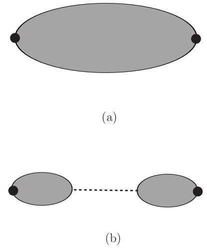
Figure 1: Diagrams contributing to $\left\langle OO\right\rangle$. (a) represents the sum of all $\phi_{2}$-connected graphs contributing to the two-point function. (b) is an example of a $\phi_{2}$-disconnected graph, where the dashed line is a $\phi_{1}$ propagator.

We can apply the general prescription for quenching to gauge theories. It is important to realize that this analysis is aimed solely at understanding the gauge-fixing procedure, and does not address the underlying mechanisms for mass generation. For simplicity, we use the language of continuum field theories, but the general form of the generating functional also holds on the lattice. Our auxiliary fields will be $g(x)$ and its partner $\widetilde{g}(x)$ which take on values in the gauge group $G.$ The Euclidean action for $g$ is simply

$$S_{g}=\int F^{2}Tr\left(D_{\mu}g\right)^{+}\left(D_{\mu}g\right)\,,$$ (19)

where the covariant derivative is $D_{\mu}g=\partial_{\mu}g+iA_{\mu}g$. The constant $F^{2}$ can be identified with $\alpha/2N$ in the lattice theory. The symmetry group is $G_{local}\otimes G_{global}$, where the gauge symmetry acts on the left, and the global symmetry acts on the right. The proxies for the gauge fields are the conserved currents associated with the global symmetry:

$$J_{\mu}^{a} = \frac{i}{2}Tr\left[gT^{a}\left(D_{\mu}g\right)^{+}-\left(Dg\right)T^{a}g^{+}\right]$$ (20)

$$= Tr\left[T^{a}g^{+}A_{\mu}g-\frac{i}{2}T^{a}g^{+}\overleftrightarrow{\partial}_{\mu}g\right].$$ (21)

If $g$ is expanded around the identity, we see the natural identification of $J_{\mu}^{a}$ as a gauge-fixed form of $A_{\mu}^{a}$.

If we couple a source $K_{\mu}^{a}$ to the currents, then the generating functional is

$$Z\left[K\right]=\int\left[dA\right]e^{-S_{A}}\frac{\int\left[dg\right]e^{-S_{g}+\int KJ}}{\int\left[d\widetilde{g}\right]e^{-S_{\widetilde{g}}}}$$ (22)

and as before, we define the generator of $g$-connected graphs to be

$$e^{W\left[K;A\right]}=\int\left[dg\right]e^{-S_{g}+\int KJ}.$$ (23)

The action $S_{g}$ can be written in the form

$$S_{g}=\int F^{2}Tr\left[\left(\partial_{\mu}g\right)^{+}\left(\partial_{\mu}g\right)+j_{\mu}A_{\mu}+A_{\mu}^{2}\right]$$ (24)

where we have defined the gauge-variant currents

$$j_{\mu}=i\left(\partial_{\mu}g^{+}\right)g-ig^{+}\partial_{\mu}g\text{ .}$$ (25)

It is important to note the distinction between $J_{\mu}$, a set of currents transforming non-trivially under the global symmetry, and the gauge-variant currents $j_{\mu}$, which transform under the local symmetry, but are invariant under the global symmetry. The generator of $g$-connected graphs is

$$e^{W\left[K;A\right]}=\int\left[dg\right]\exp\left[-\int F^{2}Tr\left[\left(\partial_{\mu}g\right)^{+}\left(\partial_{\mu}g\right)+j_{\mu}A_{\mu}+A_{\mu}^{2}-K_{\mu}J_{\mu}\right]\right]\,.$$ (26)

Now we have the expression for the proxy of the gauge field propagator

$$\left\langle J_{\mu}^{a}J_{\nu}^{b}\right\rangle=\frac{1}{Z_{A}}\int\left[dA\right]e^{-S_{A}}\left[\left(\frac{\delta^{2}W}{\delta K_{\mu}^{a}\delta K_{\nu}^{b}}\right)+\left(\frac{\delta W}{\delta K_{\mu}^{a}}\right)\left(\frac{\delta W}{\delta K_{\nu}^{b}}\right)\right]_{K=0}\,,$$ (27)

where

$$\left(\frac{\delta W}{\delta K_{\mu}^{a}}\right)_{K=0}=\frac{\int\left[dg\right]J_{\mu}^{a}\exp\left[-\int F^{2}Tr\left[\left(\partial_{\mu}g\right)^{+}\left(\partial_{\mu}g\right)+j_{\mu}A_{\mu}\right]\right]}{\int\left[dg\right]\exp\left[-\int F^{2}Tr\left[\left(\partial_{\mu}g\right)^{+}\left(\partial_{\mu}g\right)+j_{\mu}A_{\mu}\right]\right]}$$ (28)

gives rise to the graphically $g$-disconnected graphs. Similarly, the $g$-connected graphs are obtained from

$$\left(\frac{\delta^{2}W}{\delta K_{\mu}^{a}\delta K_{\nu}^{b}}\right)=\frac{\int\left[dg\right]J_{\mu}^{a}J_{\nu}^{b}\exp\left[-\int F^{2}Tr\left[\left(\partial_{\mu}g\right)^{+}\left(\partial_{\mu}g\right)+j_{\mu}A_{\mu}\right]\right]}{\int\left[dg\right]\exp\left[-\int F^{2}Tr\left[\left(\partial_{\mu}g\right)^{+}\left(\partial_{\mu}g\right)+j_{\mu}A_{\mu}\right]\right]}\,,$$ (29)

so the total propagator consists of two terms. Note that the apparent mass term for $A_{\mu}$ has been cancelled out.

In the case of QED, we can exactly solve for $\left\langle J_{\mu}J_{\nu}\right\rangle$. Writing $g$ as $\exp\left(i\theta\right)$, we have $S_{g}=\int F^{2}\left(\partial_{\mu}\theta+A_{\mu}\right)^{2}$ and the current $J_{\mu}$ is given by $J_{\mu}=A_{\mu}+\partial_{\mu}\theta$. The generating functional is

$$e^{W\left[K;A\right]}=\int\left[d\theta\right]\exp\left[-\int\frac{v^{2}}{2}\left(\partial_{\mu}\theta+A_{\mu}\right)^{2}+\int K_{\mu}\left(\partial_{\mu}\theta+A_{\mu}\right)\right]$$ (30)

where $v^{2}=2F^{2}$. Then

$$e^{W\left[K;A\right]} = \exp\left[-\int\frac{v^{2}}{2}A_{\mu}^{2}+\int K_{\mu}A_{\mu}\right]\det\left(-v^{2}\partial^{2}\right)^{-1/2}$$ (31)

$$\times\exp\left[\frac{1}{2}\int\left(K_{\mu}-v^{2}A_{\mu}\right)\frac{1}{v^{2}}\frac{\partial_{\mu}\partial_{\nu}}{\partial^{2}}\left(K_{\nu}-v^{2}A_{\nu}\right)\right]\,.$$

The momentum space form of the propagator is

$$\left\langle J_{\mu}\left(k\right)J_{\nu}\left(-k\right)\right\rangle=\left(\delta_{\mu\rho}-\frac{k_{\mu}k_{\rho}}{k^{2}}\right)\left\langle A_{\rho}\left(k\right)A_{\sigma}\left(-k\right)\right\rangle\left(\delta_{\sigma\nu}-\frac{k_{\sigma}k_{\nu}}{k^{2}}\right)+\frac{1}{v^{2}}\frac{k_{\mu}k_{\nu}}{k^{2}}\,.$$ (32)

The first term is the photon propagator, projected onto the transverse subspace, and the second term represents a direct contribution from the $\theta$ field. Note that as $v$ goes to infinity, the propagator becomes purely transverse.

It is amusing to note that the above formula is also valid in the unquenched case, where no $\widetilde{\theta}$ field is introduced. The essential change is that the gauge field acquires a mass $v$ via the simplest example of the Higgs mechanism. The propagator for $\partial_{\mu}\theta+A_{\mu}$ has exactly the same form as in the quenched case, but the mass term now causes the $A_{\mu}$ two-point function to have the explicit form

$$\left\langle A_{\rho}\left(k\right)A_{\sigma}\left(-k\right)\right\rangle=\frac{\delta_{\rho\sigma}+\frac{k_{\rho}k_{\sigma}}{v^{2}}}{k^{2}+v^{2}}$$ (33)

and one easily checks that $\left\langle J_{\mu}\left(k\right)J_{\nu}\left(-k\right)\right\rangle=\left\langle A_{\mu}\left(k\right)A_{\nu}\left(-k\right)\right\rangle$ in the unquenched case.

Lattice simulations of the $U(1)$ propagator Coddington:yz , which correspond to the limit $v\rightarrow\infty$, give a non-zero asymptotic mass in the strong-coupling, confining region, and a zero mass in the weak-coupling, free field region. In neither region are violations of spectral positivity observed, consistent with our results here.

IV Soluble Examples: Mixing Models

In our previous work Aubin:2003ih , we analyzed the simplest model displaying spectral positivity violation due to quenching: a model of two free, real scalar fields with a non-diagonal mass matrix, with one of the fields quenched. Here we generalize this to include the effects of mixing in the kinetic terms as well. The Lagrangrian for the scalar mixing model is

$$L=\frac{1}{2}\left[\left(\partial\phi_{1}\right)^{2}+m_{1}^{2}\phi_{1}^{2}\right]+\frac{1}{2}\left[\left(\partial\phi_{2}\right)^{2}+m_{2}^{2}\phi_{2}^{2}\right]-\mu^{2}\phi_{1}\phi_{2}-\varepsilon\left(\partial\phi_{1}\right)\left(\partial\phi_{2}\right)$$ (34)

where we take $\phi_{2}$ to be quenched. If $\phi_{2}$ were not quenched, this Lagrangian could be rewritten in terms of two free massive fields after a field redefinition. The quenched model can be solved by the functional method described above. We have done this in the case of $\varepsilon=0$ in Ref. Aubin:2003ih . It suffices here to note that the Dyson series for the $\phi_{2}$ propagator, truncated by quenching, is given by

$$\frac{1}{p^{2}+m_{2}^{2}}+\frac{1}{p^{2}+m_{2}^{2}}\left(\mu^{2}+\varepsilon p^{2}\right)\frac{1}{p^{2}+m_{1}^{2}}\left(\mu^{2}+\varepsilon p^{2}\right)\frac{1}{p^{2}+m_{2}^{2}}\,.$$ (35)

The $\phi_{2}$ propagator can also be written in the form

$$\allowbreak\frac{A}{p^{2}+m_{2}^{2}}+\allowbreak\frac{B}{\left(p^{2}+m_{2}^{2}\right)^{2}}+\frac{C}{p^{2}+m_{1}^{2}}\allowbreak$$ (36)

where $A$, $B$, and $C$ are functions of the parameters of the Lagrangian.

Spectral positivity is violated, because a double pole is a limiting case of a negative-metric contribution:

$$\frac{1}{\left(p^{2}+m_{2}^{2}\right)^{2}}=\lim_{m\rightarrow m_{2}}\frac{1}{m_{2}^{2}-m^{2}}\left[\frac{1}{p^{2}+m^{2}}-\frac{1}{p^{2}+m_{2}^{2}}\right].$$ (37)

The form in coordinate space is very interesting. In any number of dimensions, we can consider propagators using wall sources, i.e., sources of co-dimension $1$. This sets the momentum equal to zero in all the directions except the direction perpendicular to the wall. The coordinate space form of the two-point function is

$$\frac{A}{2m_{2}}e^{-m_{2}\left|x\right|}+\frac{B}{4m_{2}^{3}}e^{-m_{2}\left|x\right|}\left(1+m_{2}\left|x\right|\right)+\frac{C}{2m_{1}}e^{-m_{1}\left|x\right|}.$$ (38)

It is the second term, arising from the double pole, which violates spectral positivity.

Propagators are more complicated when the fields couple to both quenched and unquenched states. Consider a model of the gauge-fixed vector field as a mixture of two massive vector fields: $B_{\mu}^{a}$, which will be quenched, and $A_{\mu}^{a}$, which is unquenched. The Lagrangian density can be taken to be

$$L=\frac{1}{4}\left(\partial_{\mu}A_{\nu}^{a}-\partial_{\nu}A_{\mu}^{a}\right)^{2}+\frac{1}{4}\left(\partial_{\mu}B_{\nu}^{a}-\partial_{\nu}B_{\mu}^{a}\right)^{2}+\frac{1}{2}m_{1}^{2}\left(A_{\mu}^{a}\right)^{2}+\frac{1}{2}m_{2}^{2}\left(B_{\mu}^{a}\right)^{2}+\mu^{2}A_{\mu}^{a}B_{\mu}^{a}$$ (39)

with the sum over indices implicit. If both fields were unquenched, then the mass eigenstates would be

$$\frac{m_{1}^{2}+m_{2}^{2}\pm\sqrt{\left(m_{1}^{2}-m_{2}^{2}\right)^{2}+4\mu^{4}}}{2}.$$ (40)

Consider a field which is a linear combination of $A$ and $B$, given by $\kappa A+\lambda B$. Only the relative sign of $\kappa$ and $\lambda$ is important. The use of wall sources greatly simplifies what would be a complicated tensor structure, and the relevant Dyson series for the transverse components of the propagator is

$$\frac{\kappa^{2}}{p^{2}+m_{1}^{2}}+\frac{\lambda^{2}}{p^{2}+m_{2}^{2}}-2\frac{\kappa\lambda\mu^{2}}{\left(p^{2}+m_{1}^{2}\right)\left(p^{2}+m_{2}^{2}\right)}+\frac{\lambda^{2}\mu^{4}}{\left(p^{2}+m_{1}^{2}\right)\left(p^{2}+m_{2}^{2}\right)^{2}}$$ (41)

corresponding to the diagrams shown in Fig. 2.

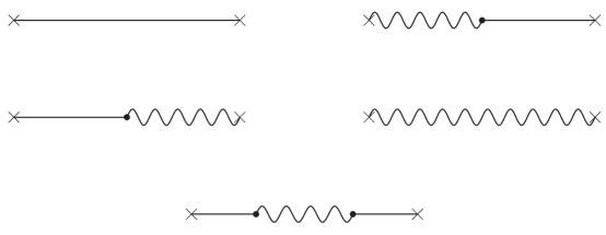
Figure 2: Diagrams that contribute to the propagator in the vector mass-mixing model. Wavy lines represent the $A_{\mu}$ propagator, and straight lines the $B_{\mu}$ propagator.

The propagator can be rearranged in several forms. The factored form

$$\frac{\lambda^{2}}{p^{2}+m_{2}^{2}}+\left(1-\frac{\lambda\mu^{2}/\kappa}{\left(p^{2}+m_{2}^{2}\right)}\right)\frac{\kappa^{2}}{p^{2}+m_{1}^{2}}\left(1-\frac{\lambda\mu^{2}/\kappa}{\left(p^{2}+m_{2}^{2}\right)}\right)$$ (42)

is helpful because it shows the beginning of the infinite Dyson series in the case where both fields are unquenched. The partial fraction form explicitly presents all the information available: there is a single pole in $p^{2}$ at $-m_{1}^{2}$, a single and a double pole at $p^{2}=-m_{2}^{2}$, and three coefficients giving the residues at the poles.

$$\left(\kappa+\frac{\lambda\mu^{2}}{m_{1}^{2}-m_{2}^{2}}\right)^{2}\frac{1}{p^{2}+m_{1}^{2}}$$

$$+\left[-\left(\frac{\lambda\mu^{2}}{\left(m_{1}^{2}-m_{2}^{2}\right)}+\kappa\right)^{2}+\lambda^{2}+\kappa^{2}\right]\frac{1}{p^{2}+m_{2}^{2}}$$

$$+\frac{\lambda^{2}\mu^{4}}{\left(m_{1}^{2}-m_{2}^{2}\right)}\frac{1}{\left(p^{2}+m_{2}^{2}\right)^{2}}\,.$$ (43)

Note that the residue of the $m_{1}$ pole must be positive, but this need not be true for the other residues, which come from the quenched fields.

V Phase Diagram of the Lattice Model

The unquenched form of the lattice model is a Higgs model, of a type first analyzed by Fradkin and Shenker Fradkin:1978dv . It is very useful to recall their analysis. For $\alpha$ and $\beta$ small, there is a convergent strong-coupling expansion associated with a phase in which the $g$ fields are confined into bound states. For $\alpha$ and $\beta$ large, perturbation theory indicates that the Higgs mechanism takes place in its most complete form, with no remaining scalar fields. At tree level, the only particles are massive vector particles. Naively, there appears to be two distinct phases, a confined phase and a Higgs phase. However, the field $g$ is in the fundamental representation of the gauge group, and breaks the $Z(N)$ symmetry associated with confinement in the pure gauge theory, in a manner similar to quarks. As Fradkin and Shenker showed, there is no absolute distinction between the confined and Higgs phases in this case, and the two regions of the lattice phase diagram are connected.

We have studied the phase diagram of the quenched model using lattice simulations, and the results are similar to those for the unquenched model. As shown schematically in Fig. 3, there is a critical line coming out of $\beta=\infty$. The origin of the line is the same in both the quenched and unquenched models: at $\beta=\infty$, the link fields become gauge transforms of the identity, and can be absorbed into the $g$ fields. Thus setting $\beta=\infty$ gives a spin model with a phase transition between a disordered phase for small $\alpha$ and an ordered phase for large $\alpha$. As $\beta$ decreases, the disordering effect of the gauge fields increases, requiring larger $\alpha$ for the phase transition. In both the quenched and unquenched cases, the critical line does not completely separate the two phases, but terminates in a critical end point in the $\alpha-\beta$ plane. This line appears to be first order in the quenched case, as is the case in the unquenched model. Figure 4 shows the specific heat for the quenched model as $\alpha$ is varied for various values of $\beta$ in the case of $SU(2)$.

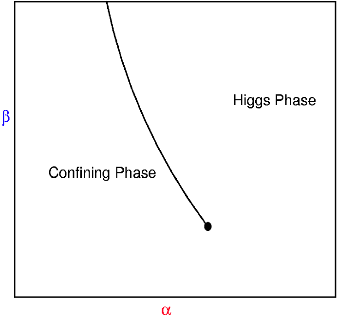
Figure 3: Phase diagram in the $\alpha-\beta$ plane for the $SU(2)$ gauge theory.

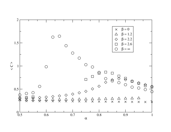
Figure 4: Plot of the specific heat for the quenched model as a function of $\alpha$.

As first discussed by Fradkin and Shenker in the unquenched case, the interpretation of the massive vector particles of the model depends on which part of the phase diagram is being considered. In the confined phase, the vector masses are associated with vector bound states of the confined scalars. This interpretation is the same in both the quenched and unquenched models. For the unquenched model, the vector particles are interpreted as fundamental particles, made massive via the Higgs mechanism. In the quenched model, this interpretation is problematic. As we have seen in our continuum treatment of gauge fixing as quenching, the term responsible for giving the vector fields a mass cancels out, and the gauge fields do not acquire a mass via the Higgs mechanism. The gauge fields can acquire a mass via their own self-interactions, however.

V.1 Interpretation as confined theory

We will interpret the vector multiplet states in the confined region in a manner similar to the work of Bardeen et al. on the $a_{0}$ in quenched QCD Bardeen:2001yz ; Bardeen:2001jm . The $\eta^{\prime}$ propagator violates spectral positivity in quenched QCD. Within chiral perturbation theory for full QCD, the $\eta^{\prime}$ becomes heavier than the particles in the pseudoscalar multiplet by the summation of a mass insertion term arising from the anomaly. In quenched QCD, the summation of the Dyson series is truncated, giving rise to a double pole in the $\eta^{\prime}$ propagator. The effects of this show up in the $a_{0}$ propagator via loops containing an $\eta^{\prime}$. The left-hand side of Fig. 5(a) shows the contribution of a single $a_{0}$ particle to the $a_{0}$ propagator, and the right-hand side shows an equivalent diagram in terms of quarks. Figures 5(b) and (c) show loop contributions from states containing an $\eta^{\prime}$ as part of the intermediate state. Figure 5(b) differs from Fig. 5(c) by a single mass insertion. In full QCD, these are the first two terms in a geometric series which can be easily summed to give a heavy $\eta^{\prime}$. In quenched QCD, Fig. 5(c) does not contribute, because it has an internal quark loop. As shown by Bardeen et al., the bubble in Fig. 5(b) leads to spectral positivity violation in the $a_{0}$ propagator.

We can take over this argument to case of gauge fixing, where the gauge-fixed vector operator must be understood as creating bound states in the confined region. In this extended analogy, there is a $g^{+}Ag$ vector bound state, whose propagation is represented by Fig. 5(a). There is also a contribution from intermediate states containing a isoscalar scalar state, as in Fig. 5(b). The isoscalar scalar thus plays a role in the confining region of the quenched theory similar to that of the $\eta^{\prime}$ in quenched QCD.

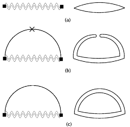
Figure 5: Diagrams contributing to the $a_{0}$ propagator in quenched QCD or the vector propagator in the confined phase of a gauge-fixing model. Diagram (c) only contributes in the unquenched case.

Let $B(p)$ stand for the bubble diagram and let the vector propagator be given by $V(p)$. We parametrize the coupling between $V$ and $B$ as $-\mu^{2}$. Suppose we look at the propagator for an operator that couples with strength $\kappa$ to the bubble and strength $\lambda$ to the vector. Then the propagator can be written in the form

$$\lambda^{2}V(p)+\left(1-\frac{\lambda\mu^{2}}{\kappa}V(p)\right)\frac{\kappa^{2}B(p)}{1+\mu^{2}B(p)V(p)}\left(1-\frac{\lambda\mu^{2}}{\kappa}V(p)\right).$$ (44)

We have chosen our parameters, including the sign of $\mu^{2}$,  to facilitate comparison with Eq. (42). If we identify the pole in the vector propagator $V(p)$ with $-m_{2}^{2}$, and the pole in the resummed bubble $\kappa^{2}B(p)/\left(1+\mu^{2}B(p)V(p)\right)$ with $-m_{1}^{2}$, then on shell we have exactly reproduced Eq. (42).

V.2 Interpretation in Higgs region

In order to discuss the region where $\alpha$ is large, we return to the continuum model of Sec. III, and write $g\left(x\right)$ as $\exp\left(iH(x)/F\right)$ where $H$ is Hermitian and traceless. We assume that for $F$ sufficiently large, we are in the Higgs phase, where $g\left(x\right)$ can be expanded around the identity. We are only treating $g\left(x\right)$ perturbatively, and non-perturbative phenomena in the gauge-field sector, such as dynamical mass generation, are not treated here.

In the unquenched theory, the Higgs mechanism would occur via the term in $S_{g}$

$$\int F^{2}Tr\left(A_{\mu}g\right)^{+}\left(A_{\mu}g\right)=\int F^{2}TrA_{\mu}^{2}\,,$$ (45)

but this term is explicitly canceled in the quenched theory. Internal loops associated with $H$ are also cancelled out in the quenched theory, as discussed in Sec. III. The gauge-invariant current $J_{\mu}^{a}$, which is a proxy for the gauge field, is

$$J_{\mu}^{a} = Tr\left[T^{a}g^{+}A_{\mu}g-\frac{i}{2}T^{a}g^{+}\overleftrightarrow{\partial}_{\mu}g\right]$$ (46)

$$= Tr\Biggl{[}T^{a}\biggl{(}A_{\mu}-\frac{i}{F}\left[H,A_{\mu}\right]+\frac{1}{F}\partial_{\mu}H-\frac{1}{2F^{2}}\left[H,\left[H,A_{\mu}\right]\right]$$

$${}-\frac{i}{2F^{2}}\left[H,\partial_{\mu}H\right]\biggr{)}+O(H^{3})\Biggr{]}\,,$$

so the current $J_{\mu}^{a}$ has a term with $A_{\mu}^{a}$ alone. On the other hand, the current which couples perturbatively to $A_{\mu}$ is

$$j_{\mu} = i\left(\partial_{\mu}g^{+}\right)g-ig^{+}\partial_{\mu}g$$ (47)

$$= \frac{2}{F}\partial_{\mu}H+\frac{i}{F^{2}}\left[\partial_{\mu}H,H\right]+O(H^{3})$$

so that $J_{\mu}$ and $j_{\mu}$ have some common terms.

The propagator $\left\langle J_{\mu}^{a}J_{\nu}^{b}\right\rangle$ is given by Eq. (27)

$$\left\langle J_{\mu}^{a}J_{\nu}^{b}\right\rangle=\int\left[dA\right]e^{-S_{A}}\left[\left(\frac{\delta^{2}W}{\delta K_{\mu}^{a}\delta K_{\nu}^{b}}\right)+\left(\frac{\delta W}{\delta K_{\mu}^{a}}\right)\left(\frac{\delta W}{\delta K_{\nu}^{b}}\right)\right]_{K=0}.$$

The first term represents $g$-connected graphs, as shown in Fig. 6(a). The second term represents all other contributions, including intermediate states involving one or more $A_{\mu}$ propagators. If we assume that the intermediate state with one $A_{\mu}$ propagator dominates, then we need only consider the graphs shown in Fig. 6(b)-(e). The sum of graphs has the same structure seen in the confined phase.

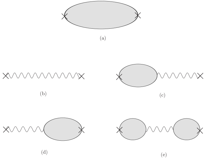
Figure 6: Schematic diagrams contributing to the vector propagator in the Higgs phase. (a) consists of all $g$-connected contributions, while (b)-(e) are the $g$-disconnected pieces with single gluon exchange.

Comparison of Fig. 6 with Eq. (42) immediately suggests that the double pole associated with the mass $m_{2}$ can be understood as arising from Fig. 6(e). This does not fix the origin of the $m_{1}$ pole. One possibility is that $m_{1}$ is associated with Fig. 6(b), in which case $m_{1}$ would be a candidate for what we mean by the term gluon mass. As we will see in the next section, lattice simulations indicate that the mass $m_{1}$ is too heavy to represent a phenomenologically realistic gluon mass. Another possibility is that both the $m_{1}$ and $m_{2}$ poles occur in Fig. 6(a), as happens in the confined region. From this point of view, the diagrams in Fig. 5(a) and (b), which are both $g$-connected, could move smoothly into Fig. 6(e). Thus the interpretation of the masses is ambiguous in this phase.

VI Lattice Results for Propagators

We have performed simulations with the action in Eq. (5) for the case of $SU(2)$ $20^{4}$ lattices at $\beta=2.4$ and $\alpha=\left\{1,1.2,1.4,1.6,1.75,2.0,2.5,3.0\right\}$. The critical line in the $\left(\alpha,\beta\right)$ plane lies near $\alpha=0.8$, so most of these points are well inside the Higgs region of the phase diagram. For each value of $\alpha$, we have performed four independent simulations. Fits were carried out for each dataset, and finally combined to give final results for the fitting parameters. We begin the analysis in coordinate space to extract the masses from the form

$$G(x)=(a+bm_{2}x)e^{-m_{2}x}+ce^{-m_{1}x}+(x\rightarrow L-x)\ .$$ (48)

In order to extract the masses, we first cut the data at $x=x_{0}$, and fit the term $(a+bm_{2}x)e^{-m_{2}x}+(x\rightarrow L-x)$ to all points $x\geq x_{0}$. The value of $x_{0}$ is chosen to achieve the best fit, and depends on the dataset, but in all cases $x_{0}>1/m_{1}$. This then gives us a value for the mass $m_{2}$ (and $a$ and $b$). Once this has been fit, we subtract this from the original data set and then fit the remainder to $ce^{-m_{1}x}+(x\rightarrow L-x)$ to extract the mass $m_{1}$, as well as $c$.

The coordinate space form of the propagator is sufficient for the determination of the two mass parameters. The coefficients $\kappa$, $\lambda$, and $\mu^{2}$ are complicated functions of $a$, $b$ and $c$ in the coordinate space propagator. Thus it is easiest to extract the mass parameters $m_{1}$ and $m_{2}$ in coordinate space, but determine the other parameters in momentum space. After Fourier transforming the propagators, we multiply by the factor $(p^{2}+m_{2}^{2})^{2}(p^{2}+m_{1}^{2})$, where $p^{2}$ should be understood as the one-dimensional lattice momentum squared, $\sin^{2}(p)$. We then fit $(p^{2}+m_{2}^{2})^{2}(p^{2}+m_{1}^{2})G(p)$ to a quadratic polynomial in $p^{2}$. The coefficients of the polynomical can be extracted cleanly, and from these we can determine the parameters from Eq. (41), $\mu^{2}$, $\kappa$ and $\lambda$. Empirically, we find that these parameters are only weakly dependent on the mass parameters. Finally we have taken the values found with these fitting routines and have averaged over the four sets of data for each value of $\alpha$, where the error bars are determined from calculating the standard error as these data are statistically independent.

In Figs. 7 and 8 we compare our $20^{4}$ propagator results with our earlier work Aubin:2003ih on a $12^{3}\times 16$ lattice at $\beta=2.4$ for the values $\alpha=1.2$ and $2.0$ respectively. Errors are smaller than the size of the data points. The consistency of the data and the absence of any finite-size effects is clear, as expected from the magnitude of the masses.

In Figs. 9 and 10 we plot $m_{1}$ and $m_{2}$ as a function of $\alpha$ on both $12^{3}\times 16$ and $20^{4}$ lattices. We note that $m_{2}$ appears to be essentially independent of $\alpha$ over the range studied, and the results from the two lattice sizes are quite consistent. The mass parameter $m_{1}$ shows definite $\alpha$ dependence for smaller values of $\alpha$. The disagreement in the results for $m_{1}$ for the two lattice sizes is not statistically significant, but $m_{1}$ is clearly not as well-determined as $m_{2}$. This is to be expected, since $m_{1}$ is much larger than $m_{2}$, and is extracted from the same propagator.

The parameters $\kappa$, $\lambda$, and $\mu^{2}$ are shown as functions of $\alpha$ in Figs. 11-13. The parameter $\kappa$ represents the coupling of the lattice gluon operator to the unquenched particle, which has mass $m_{1}$. It is monotonically decreasing as a function of $\alpha$, but it is difficult to determine if it asymptotes to a non-zero value for large $\alpha$. The parameter $\lambda$ is the coupling of the gluon operator to the quenched particle, which has mass $m_{2}$. This parameter is not as well-determined as $\kappa$, but is much larger for large $\alpha$. The parameter $\mu^{2}$, which represents the mixing of the quenched and unquenched particles, show a downward trend with increasing $\alpha$, but with large statistical errors.

The behavior of the two masses $m_{1}$ and $m_{2}$ as functions of $\alpha$ are completely different from the behavior of the vector particle in the unquenched model. As shown in Fig. 14, the vector mass $m_{V}$ in the unquenched model rises as $\alpha^{1/2}$ over this range of $\alpha$, all at $\beta=2.6$. The unquenched propagator fits very well to a single pole form in this region. This is completely consistent with the Higgs interpretation of the unquenched model, where $m_{V}^{2}$ is naively proportional to $\alpha$ in physical gauge. Suppose for the moment that we were simulating the mixing model instead of an $SU(2)$ gauge theory. Then the parameters $m_{1}$, $m_{2}$, and $\mu$ from the quenched simulation could be used to determine the mass eigenstates via Eq. (40). This procedure is dubious for the gauge theory, because only one multiplet of vector mass eigenstates occurs in the unquenched model, not two. Furthermore, the parameters of the quenched and unquenched models are different due to quenching. Nevertheless, if the parameters of the unquenched model are used in Eq. (40), the larger of the two masses is commensurate with the single mass observed in the unquenched model.

Our analysis of the gluon propagator reveals three parameters with dimensions of mass: $m_{1}$, $m_{2}$, and $\mu$. As we have discussed above, there are arguments for both $m_{1}$ and $m_{2}$ to be interpreted as a gluon mass parameter. The mass $m_{1}$ is the mass of the unquenched state, and it is natural to assume that it is the gluon mass. However, the mass of the lightest glueball in $SU(2)$ is given by $m_{G}/\sqrt{\sigma}=3.74\pm 0.12$ Teper:1998kw , and $a\sqrt{\sigma}=0.1326$, so $m_{G}a=0.4959$. Thus $m_{1}$ is about $2m_{G}$, and is an unlikely candidate for a gluon mass.

On the other hand, $m_{2}$ is slightly larger than $m_{G}/2$. If we view the lightest scalar glueball as being composed of two consituent gluons, then it is natural to identify $m_{2}$ as the gluon mass. Furthermore, $m_{2}$ is the lightest mass in the vector channel, and it is logical to identify this with the gluon. In the confined phase interpretation of the unquenched model, the lightest vector is a bound state of a gluon, scalar, and anti-scalar. In the Higgs phase, the lightest vector is simply the massive vector particle formed by the Higgs mechanism. We expect that any meaningful gluon mass would be independent of $\alpha$, and $m_{2}$ appears to be approximately constant over the range of $\alpha$ studied.

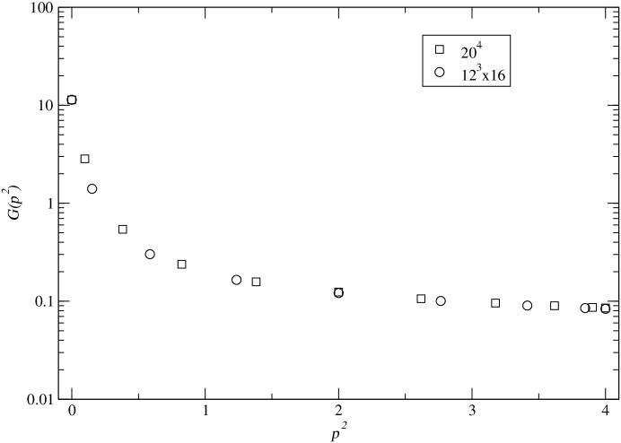
Figure 7: The momentum space gluon propagator on the $12^{3}\times 16$ and $20^{4}$ lattices at $\alpha=1.2$.

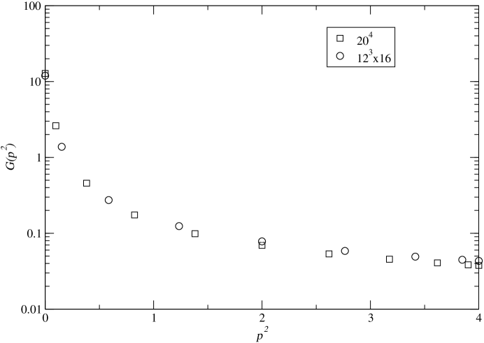
Figure 8: The momentum space gluon propagator on the $12^{3}\times 16$ and $20^{4}$ lattices at $\alpha=2.0$.

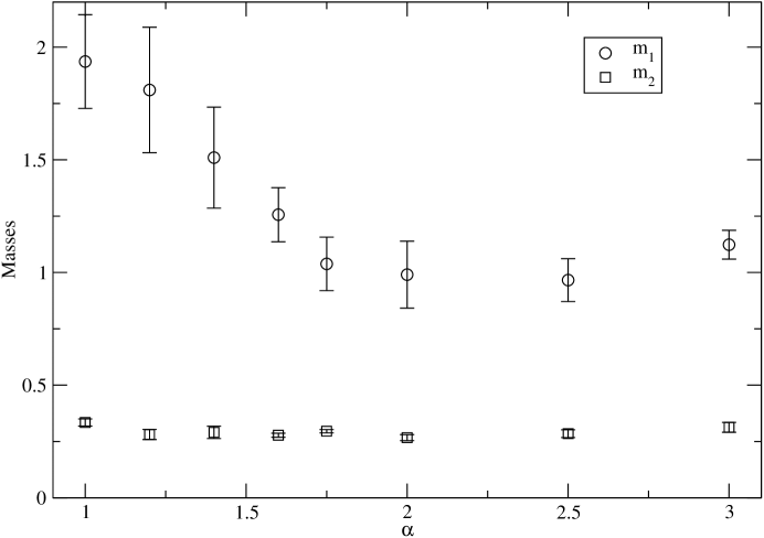
Figure 9: Values of the two mass parameters in as a function of $\alpha$ on the $12^{3}\times 16$ lattice. The light mass, $m_{2}$ is approximately constant as a function of $\alpha$, while the heavy mass initially decreases with increasing $\alpha$, reaching a somewhat constant value.

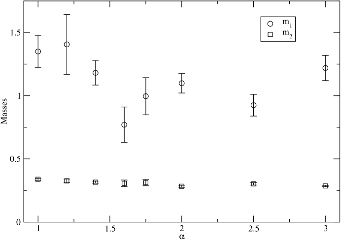
Figure 10: Same as Fig. 9, but for the $20^{4}$ lattice.

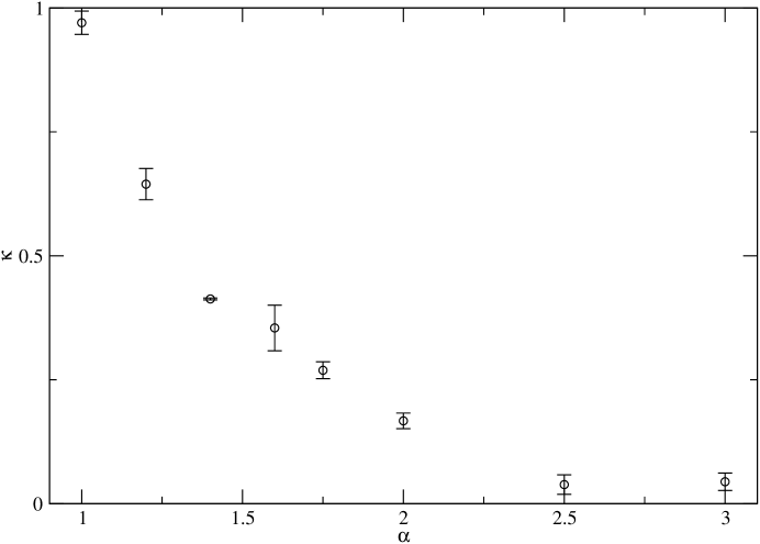
Figure 11: $\kappa$ as a function of $\alpha$.

Figure 12: $\lambda$ as a function of $\alpha$.

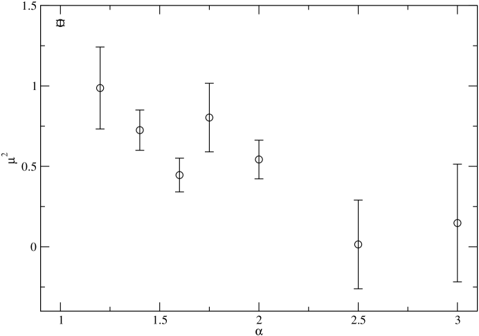
Figure 13: $\mu^{2}$ as a function of $\alpha$.

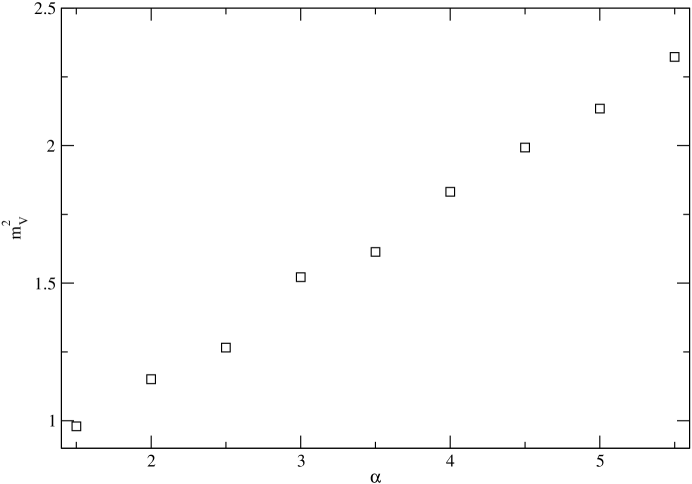
Figure 14: The mass-squared determined from fitting the gluon propagator in the unquenched theory to a single pole form. The linear trend is obvious.

VII Discussion

A large number of possible forms for the gluon propagator, in various gauges, have been proposed. A brief review is available in Ref. Mandula:nj . We confine ourselves here to a few remarks on some of the main themes that have been considered in the literature. We begin by noting that there is no evidence from lattice simulations for massless excitations coupled to the gluon propagator. In particular, a $1/p^{4}$ propagator, which would lead to a confining potential from one-gluon exchange Mandelstam:1979xd , is firmly ruled out.

The possibility that the gluon propagator might vanish at zero momentum was first discussed by Gribov, based on his work on gauge copies Gribov:1977wm . He proposed that the gluon propagator has complex poles, leading to a gluon propagator of the form

$$\frac{p^{2}}{p^{4}+m^{4}}.$$ (49)

This leads to the vanishing of the gluon propagator at $p=0$, and a peak in the gluon propagator at a non-zero momentum. Others have also explored this possibility and possible generalizations Cucchieri:2000kw ; vonSmekal:1997is . Zwanziger has proven Zwanziger:gz that the gluon propagator in lattice Landau gauge ($\alpha=\infty$) is zero at $p^{2}=0$ in the infinite volume limit. His proof does not require the continuum limit, but does require that only configurations in a restricted region of configuration space, such as the fundamental modular region, be integrated over. There is evidence from some lattice simulations for a peak in the gluon propagator at very low wave number Cucchieri:2000kw ; Cucchieri:2003di . However, extremely large lattices are required, and the propagator does not appear to be trending to zero at $p^{2}=0$ as the volume grows.

In our lattice simulations, the gluon propagator does not vanish at $p^{2}=0$ and our best fit to the data does not indicate a peak to non-zero momentum. However, within the framework of our mixing model, it is possible for a peak to occur, depending on the values of various parameters. If the gluon propagator is initially rising with $p^{2}$, it must eventually fall. Thus the condition for a peak to occur is

$$2m_{1}^{2}\kappa\lambda\mu^{2}m_{2}^{2}-2m_{1}^{2}\lambda^{2}\mu^{4}-m_{1}^{4}\lambda^{2}m_{2}^{2}+2m_{2}^{4}\kappa\lambda\mu^{2}-m_{2}^{2}\lambda^{2}\mu^{4}-m_{2}^{6}\kappa^{2}>0.$$ (50)

Our measured parameters are such that this inequality never holds. We have also fit our data with the form used by Cucchieri et al. in Ref. Cucchieri:2000kw , a generalization of the Gribov form. Although a reasonable fit to the data is obtained, the $\chi^{2}$ is 50-100 times larger than that obtained with our quenched mixing form, and a peak is not always seen. When a peak does appear when fitting to the generalized Gribov form, it occurs at very small non-zero momenta, directly accessible only on very large lattices. We conclude that a peak is a possible feature of the gluon propagator, but the existence of a peak is sensitive to the precise form used in fitting. Such a peak may lack fundamental significance, particularly since it may only be directly observable on lattices much larger than the scale on which confinement appears.

Our results for the gluon propagator are similar to those of Leinweber et al. Leinweber:1998uu , who fit $SU(3)$ lattice Landau gauge propagators to a variety of possible forms. They obtain a best fit with their model A, for which the propagator has the form

$$D\left(p^{2}\right)=Z\left[\frac{AM^{2\alpha_{L}}}{\left(p^{2}+M^{2}\right)^{1+\alpha_{L}}}+\frac{L(p^{2},M^{2})}{p^{2}+M^{2}}\right]$$ (51)

where $L$ is a logarithmic factor mimicking one-loop corrections. Their preferred value for their parameter $\alpha_{L}$ is $2.17_{-19}^{+11}$. This form is thus rather similar to our quenched mixing form, since for $\alpha_{L}=2$, it has a triple pole. Of course, we have two mass scales, $m_{1}$ and $m_{2}$, playing roles in the denominators.

We have not explored the interesting possibility that the gluon propagator has an anomalous dimension, first suggested by Marenzoni et al. Marenzoni:td . This behavior could occur in our formulation. For example, the bubble diagram discussed in Sec. V could give this behavior. However, high precision data as well as a detailed functional form for fitting would be needed to test for this behavior.

VIII Conclusions

We have shown in detail how the quenched character of lattice gauge fixing leads to violations of spectral positivity in non-Abelian gauge theories. Although we have focused on lattice Landau gauge, this problem is likely to occur in any lattice gauge fixing scheme in which the gauge fixing variables are determined subsequent to the generation of lattice gauge field configurations. A key step in our analysis has been the generalization of conventional lattice gauge fixing, where one configuration is chosen on the gauge orbit, to a formalism including a gauge-fixing parameter, similar to continuum gauge fixing. This parameter controls the weighting of configurations along the gauge orbit, and conventional lattice gauge fixing is formally recovered as a limiting case. We have not examined lattice gauge fixing schemes in which the gauge field integration is restricted to a subset of the entire configuration space, e.g., the fundamental modular domain, but the relation of these to standard computational practice is unclear. There are some lattice gauge fixing schemes, such as lattice Laplacian gauge Vink:1992ys which are defined by a complicated algorithmic process, and may not generalize in a manner similar to lattice Landau gauge. Nevertheless, we believe that the quenched character of these algorithms is the root of spectral positivity violation there as well.

We have focused here on the form of the gluon propagator, the extraction of masses, their interpretation and dependence on the gauge-fixing parameter $\alpha$. The issue of the continuum limit for gluon propagator masses has not yet been resolved. In the gauge-invariant sector, physical masses scale as the gauge coupling $\beta$ is taken to infinity in the manner prescribed by the renormalization group. In principle, it is also necessary to adjust $\alpha$ to obtain a continuum limit of gauge-variant quantities. In other words, the running of the gauge-fixing parameter must be taken into account. This is similar to the running of the gauge-fixing parameter in covariant gauges in the continuum. If a meaningful gluon mass, independent of $\alpha$ for large $\alpha$, can be extracted, it might scale correctly in the continuum limit without tuning $\alpha$. As we have observed, the mass $m_{2}$ is approximately independent of $\alpha$ for large $\alpha$ at $\beta=2.6$, and has a value phenomenologically consistent with a constituent gluon mass. Further study is required to see if $m_{2}$ and $m_{1}$ survive in the continuum limit. Because the standard gluon operator creates a mixture of states, it is likely that a variational analysis Albanese:ds ; Teper:wt using a several operators would give a better determination of $m_{2}$ and particularly $m_{1}$.

We have used the group $SU(2)$ to study gluon properties at zero temperature. Perhaps the most important application of lattice gauge fixing is the measurement of electric and magnetic masses in the deconfined phase. We are extending our work to finite temperature $SU(2)$, generalizing the work of Refs. Heller:1995qc ; Heller:1997nq ; Cucchieri:2000cy to the case of finite $\alpha$. However, it is $SU(3)$ which is of principal interest Nakamura:2003pu . Because gauge fixing can be carried out any time after lattice field configurations are generated, it is relatively easy to study gauge fixing on available unquenched $SU(3)$ configurations. In that case, it would be possible to also examine the dependence of the quark mass on the gauge parameter $\alpha$.

References

- (1) J. Greensite, Prog. Part. Nucl. Phys. 51, 1 (2003) [arXiv:hep-lat/0301023].
- (2) J. E. Mandula, Phys. Rept. 315, 273 (1999).
- (3) U. M. Heller, F. Karsch and J. Rank, Phys. Lett. B 355, 511 (1995) [arXiv:hep-lat/9505016].
- (4) U. M. Heller, F. Karsch and J. Rank, Phys. Rev. D 57, 1438 (1998) [arXiv:hep-lat/9710033].
- (5) A. Cucchieri, F. Karsch and P. Petreczky, Phys. Lett. B 497, 80 (2001) [arXiv:hep-lat/0004027].
- (6) A. Nakamura, T. Saito and S. Sakai, Phys. Rev. D 69, 014506 (2004) [arXiv:hep-lat/0311024].
- (7) J. E. Mandula and M. Ogilvie, Phys. Lett. B 185, 127 (1987).
- (8) P. Coddington, A. Hey, J. Mandula and M. Ogilvie, Phys. Lett. B 197, 191 (1987).
- (9) C. Parrinello and G. Jona-Lasinio, Phys. Lett. B 251, 175 (1990).
- (10) D. Zwanziger, Nucl. Phys. B 345, 461 (1990).
- (11) S. Fachin and C. Parrinello, Phys. Rev. D 44, 2558 (1991).
- (12) D. S. Henty, O. Oliveira, C. Parrinello and S. Ryan [UKQCD Collaboration], Phys. Rev. D 54, 6923 (1996) [arXiv:hep-lat/9607014].
- (13) M. C. Ogilvie, Phys. Rev. D 59, 074505 (1999) [arXiv:hep-lat/9806018].
- (14) C. A. Aubin and M. C. Ogilvie, Phys. Lett. B 570, 59 (2003) [arXiv:hep-lat/0306012].
- (15) V. K. Mitrjushkin and A. I. Veselov, JETP Lett. 74, 532 (2001) [Pisma Zh. Eksp. Teor. Fiz. 74, 605 (2001)] [arXiv:hep-lat/0110200].
- (16) L. Giusti, M. L. Paciello, C. Parrinello, S. Petrarca and B. Taglienti, Int. J. Mod. Phys. A 16, 3487 (2001) [arXiv:hep-lat/0104012].
- (17) W. Bock, M. Golterman, M. Ogilvie and Y. Shamir, Phys. Rev. D 63, 034504 (2001) [arXiv:hep-lat/0004017].
- (18) S. Elitzur, Phys. Rev. D 12, 3978 (1975).
- (19) E. H. Fradkin and S. H. Shenker, Phys. Rev. D 19, 3682 (1979).
- (20) W. A. Bardeen, A. Duncan, E. Eichten, N. Isgur and H. Thacker, Nucl. Phys. Proc. Suppl. 106, 254 (2002) [arXiv:hep-lat/0110187].
- (21) W. A. Bardeen, A. Duncan, E. Eichten, N. Isgur and H. Thacker, Phys. Rev. D 65, 014509 (2002) [arXiv:hep-lat/0106008].
- (22) M. J. Teper, arXiv:hep-th/9812187.
- (23) S. Mandelstam, Phys. Rev. D 20, 3223 (1979).
- (24) V. N. Gribov, Nucl. Phys. B 139, 1 (1978).
- (25) A. Cucchieri and D. Zwanziger, Phys. Lett. B 524, 123 (2002) [arXiv:hep-lat/0012024].
- (26) L. von Smekal, R. Alkofer and A. Hauck, Phys. Rev. Lett. 79, 3591 (1997) [arXiv:hep-ph/9705242].
- (27) D. Zwanziger, Nucl. Phys. B 364, 127 (1991).
- (28) A. Cucchieri, T. Mendes and A. R. Taurines, Phys. Rev. D 67, 091502 (2003) [arXiv:hep-lat/0302022].
- (29) D. B. Leinweber, J. I. Skullerud, A. G. Williams and C. Parrinello [UKQCD Collaboration], Phys. Rev. D 60, 094507 (1999) [Erratum-ibid. D 61, 079901 (2000)] [arXiv:hep-lat/9811027].
- (30) P. Marenzoni, G. Martinelli, N. Stella and M. Testa, Phys. Lett. B 318, 511 (1993).
- (31) J. C. Vink and U. J. Wiese, Phys. Lett. B 289, 122 (1992) [arXiv:hep-lat/9206006].
- (32) M. Albanese et al. [APE Collaboration], Phys. Lett. B 192, 163 (1987).
- (33) M. Teper, Phys. Lett. B 183, 345 (1987).