HU-EP-04/27
SFB/CPP-04-15

Impact of large cutoff–effects on algorithms
for improved Wilson fermions

Abstract

As a feasibility study for a scaling test we investigate the behavior of algorithms for dynamical fermions in the $N_{f}\!=\!2$ Schrödinger functional at an intermediate volume of $1\,{\rm fm}^{4}$. Simulations were performed using HMC with two pseudo–fermions and PHMC at lattice spacings of approximately $0.1$ and $0.07\,{\rm fm}$. We show that some algorithmic problems are due to large cutoff–effects in the spectrum of the improved Wilson–Dirac operator and disappear at the smaller lattice spacing. The problems discussed here are not expected to be specific to the Schrödinger functional.

1 Introduction

1.1 Motivation

For improved Wilson fermions it has long been established that in the quenched approximation cutoff–effects at a lattice spacing of $a\!\simeq\!0.1\,{\rm fm}$ are tolerable and a continuum extrapolation can be started there. Recently more and more evidence has been accumulated that for dynamical improved Wilson fermions in a similar physical condition the cutoff–effects are much larger than expected. As an extreme example, for three flavors the existence of a phase transition in the $\beta$–$\kappa$–plane has been numerically conjectured and is interpreted as a lattice artifact [?]. A summary of large scaling violations in the two–flavor–theory is given in ref. [?].

In order to quantify those we are preparing a scaling test similar to what was done for the quenched case in ref. [?]. This will also serve as a benchmark for new actions. In the course of the scaling study we plan to calculate the axial current normalization constant $Z_{\rm A}(g_{0}^{2})$ and the axial current improvement constant $c_{\rm A}(g_{0}^{2})$ using the methods described in refs. [?] and [?], respectively.

On our coarser lattices we encountered algorithmic difficulties in both the molecular dynamics integration of the Hybrid Monte Carlo (HMC) and the efficient simulation of the canonical ensemble. We thus found it advantageous to deviate from importance sampling. Here we will discuss these problems and their link to cutoff–effects at the infrared end of the spectrum of the Dirac operator.

This paper is organized as follows: In the remainder of Section 1 we will briefly describe our setup and give a summary of the parameters of the simulations, which we will quote in the following sections. In Section 2 we describe in more detail the problems encountered at large coupling and also discuss methods to address these. In this context we study the behavior of the Polynomial Hybrid Monte Carlo (PHMC) algorithm [?,?] in this situation and find it a very useful tool for a detailed investigation of the properties of the small eigenvalues of the Dirac operator.

Section 3 is devoted to a comparison of the spectrum with the quenched case at matched physical parameters and in Section 4 we present results from an exploratory run at a smaller lattice spacing. We close with a brief summary of our findings.

1.2 Setup

All our simulations were performed in the Schrödinger functional (SF) setup [?,?]. We use non–perturbatively improved Wilson fermions [?,?,?,?] and the plaquette gauge action. For $N_{f}\!=\!2$ the clover coefficient $c_{\rm SW}$ at $\beta\!=\!5.2$ has been set to the value suggested in [?] and recently confirmed by the JLQCD Collaboration [?]. For the additional boundary–improvement coefficients needed in the SF we used the perturbative values for $c_{t}$ (2–loop) [?] and $\tilde{c}_{t}$ (1–loop) [?]. The axial current improvement constant $c_{\rm A}$ is also set to its 1–loop value [?]. The first algorithm used is the HMC with two pseudo–fermion fields as proposed in ref. [?]. We want to note that the physical situation here is quite different from the one where this algorithm was previously applied and its performance tested by the ALPHA Collaboration [?]. In our planned scaling study we are interested in intermediate size physical volumes and lattice spacings between $0.1$ and $0.05\,{\rm fm}$. As mentioned above the second algorithm we employed is the PHMC, which we will discuss in some detail in Section 2. Apart from global sums all our calculations are carried out in single–precision arithmetics.

1.3 Simulation parameters

In Table 1 we list the lattice sizes and bare parameters of our simulations. In all cases we have $T\!=\!9/4\;L$ for the time extension $T$. The bare quark mass $m$ is defined in the appendix of ref. [?]. In the algorithm column ’$\rm H_{2}$’ refers to HMC with two pseudo–fermion fields and ’$\rm P_{n}$’ stands for PHMC with a polynomial of degree $n$. The trajectory length is always equal to one and the molecular dynamics integration step–size is denoted by $\delta\tau$. For each simulation we ran 16 independent replica to gain more statistics. Concerning the SF parameters we work with zero background field and periodic spatial boundary conditions ($\theta\!=\!0$).

run	$L/a$	$\beta$	$\kappa$	$c_{\rm SW}$	$\ \ Lm$	algo.	$N_{\rm traj}$	$\delta\tau$	acc.
I	8	5.2	0.13550	2.017	0.205(10)	$\,\rm H_{2}$	$16\!\cdot\!500$	1/16	91%
II	8	5.2	0.13515	2.017	0.307(9)	$\,\rm H_{2}$	$16\!\cdot\!520$	1/25	97%
III	8	5.2	0.13515	2.017	0.314(8)	$\,\rm P_{140}$	$16\!\cdot\!500$	1/26	87%
IV	8	5.2	0.13550	2.017	0.195(7)	$\,\rm P_{140}$	$16\!\cdot\!400$	1/25	85%
V	8	6.0	0.13421	1.769	0.193(3)	— quenched —
VI	12	5.5	0.13606	1.751	0.287(3)	$\,\rm H_{2}$	$16\!\cdot\!240$	1/20	91%
VII	12	6.26	0.13495	1.583	0.295(3)	— quenched —

Table 1: Summary of simulation parameters.

2 Sampling problems on coarse lattices

2.1 Instabilities in the molecular dynamics integration

Algorithms making use of molecular dynamics (MD) require a numerical integration of the equations of motion. Along a trajectory the Hamiltonian is then only conserved up to powers of the step–size $\delta\tau$ employed in the integration. Apart from these small deviations, under certain conditions the currently used integration schemes can become unstable and produce very large Hamiltonian violations $\Delta H$. For a more detailed discussion see ref. [?], where a connection between these instabilities and large driving forces in the MD is proposed in analogy to a harmonic oscillator model. In this model the integrator becomes unstable when the product of the force and the integration step–size exceeds a certain value.

The reversibility of the numerical integration is needed to prove detailed balance for these algorithms, which in turn implies that $\langle e^{-\Delta H}\rangle\!=\!1$. Here one should note that the average is taken over all proposed configurations (see ref. [?]). Therefore this quantity is also sensitive to those, which were rejected in the Metropolis step following the MD integration, i.e. trajectories resulting in a large value of $\Delta H$. In a histogram of $e^{-\Delta H}$ these contribute to bins close to zero while the distribution is peaked around one. They can also lead to an unusual autocorrelation of this quantity, making the Monte Carlo error estimate difficult. In particular this applies also to the integrated autocorrelation time of $e^{-\Delta H}$ itself. This is due to the long periods of rejection in the Metropolis step, which sometimes follow large $\Delta H$ values.

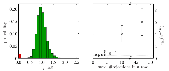
Figure 1: $e^{-\Delta H}$ from run I. Left plot: histogrammed distribution. Right plot: our estimates of $\tau_{\rm int}$ in units of MD time separately for the 16 replica. In our normalization $\tau_{\rm int}=0.5$ means no autocorrelation (dotted line).

Fig. 1 shows a histogram of $e^{-\Delta H}$ and also its integrated autocorrelation time from one of our simulations. In this data set there are several series of large $\Delta H$ values, during which the proposed configurations were rejected. In the distribution of $e^{-\Delta H}$ these lead to an additional peak close to zero. One also sees from the right–hand plot that $e^{-\Delta H}$ is noticeably autocorrelated only when a large number of proposals were rejected in a row. As argued above in these cases the error of $\tau_{\rm int}$ could be underestimated. These two effects might cause some concerns when using $\langle e^{-\Delta H}\rangle-1$ as an indicator for the absence of reversibility violations [?].

Spikes in $\Delta H$ have been observed by several collaborations using (improved) Wilson fermions in various setups (e.g. different gauge actions and volumes) at relatively large lattice spacings [?,?,?,?]. There these spikes have been traced back to large values of the driving force in the MD evolution and also their dependence on the quark mass has been investigated.

Here we want to clarify a point, which is essentially implied by the previous observations [?,?], namely the strong correlation between spikes in $\Delta H$ and small eigenvalues of the Dirac operator. In this way we hope to be able to separate physical effects from cutoff–effects, i.e. the occurrence of unphysically small eigenvalues. In Fig. 2 we clearly see a long period of rejection (corresponding to the rightmost data point in Fig. 1) caused by the presence of a very small eigenvalue. Although we did not measure them, this is expected to produce large fermionic contributions to the driving forces since they involve an inverse power of the Dirac operator.

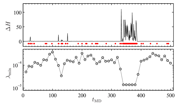
Figure 2: Monte Carlo history for one replicum of run I with a long period of rejection. Configurations where the new proposal was rejected are marked by a dot. At $t_{\rm MD}\!\!=\!340$ the algorithm gets stuck with a configuration carrying an exceptionally low smallest eigenvalue $\lambda_{\rm min}$ of $\hat{Q}^{2}$.

We found the observed average $\lambda_{\rm min}$ to be close to its tree–level estimate with Schrödinger functional boundary conditions [?]. However, the smallest $\lambda_{\rm min}$ is an order of magnitude below that and we therefore consider these eigenvalues unphysical and will later establish their nature as cutoff–effects.

Finally, following the procedure of ref. [?], the absence of global reversibility violations is explicitly verified even for trajectories resulting in large values of $\Delta H$. Nevertheless our experience shows that the increased cost of using a smaller $\delta\tau$ such that no long periods of rejection occur is more than compensated by the reduction in autocorrelation time of all observables. The reason is that already a small decrease of the integration step–size greatly reduces the Hamiltonian violations. For example, repeating run I with a step–size of $1/20$ instead of $1/16$, the longest period of rejection was $4$ (instead of $47$) consecutive trajectories.

2.2 MC estimates of fermionic observables

We concluded in the previous section that unphysically small eigenvalues of $\hat{Q}^{2}$ produce algorithmic problems only on a practical and not on a theoretical level. But apart from slowing down the algorithm these small eigenvalues also cause problems in the MC evaluation of fermionic Green’s functions.

Consider the Schrödinger functional correlation function $f_{1}$ as defined in ref. [?]. It is the correlation between pseudo–scalar composite fields at the first and last time–slice, respectively. We will denote its value on a given gauge field configuration by ${[\phi_{1}]_{\rm F}}$.

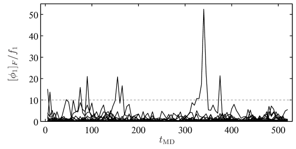
Figure 3: Monte Carlo history for the $N_{\rm rep}\!=\!16$ replica of run II showing the normalized ${[\phi_{1}]_{\rm F}}$.

Fig. 3 shows the MC history of the normalized ${[\phi_{1}]_{\rm F}}$ for the 16 replica of run II. Here $t_{\rm MD}$ refers to the molecular dynamics time for each replicum. While on this scale the bulk of the data are below one and hence not visible there are several peaks, which have a big influence on the mean value. These spikes also affect the error estimate $\sigma(f_{1})$ through both the variance and the integrated autocorrelation time [?]. For statistically accessible quantities the error should approach a $1/\sqrt{t_{\rm MD}}$ behavior in the limit $t_{\rm MD}\!\rightarrow\!\infty$. In this respect we found $f_{1}$ and all other fermionic correlation functions we considered to be very hard to measure. Even when using $16$ replica, this asymptotic behavior does not set in after $t_{\rm MD}\!\simeq\!500$.

The reason is the rare occurrence of very large values of ${[\phi_{1}]_{\rm F}}$, which appear to be correlated with small eigenvalues of $\hat{Q}^{2}$. However, this effect is washed out by using several replica. We therefore show in Fig. 4 the MC history of ${[\phi_{1}]_{\rm F}}$, $\lambda_{\rm min}$ and our error estimate for $f_{1}$ for one replicum of run II with such a spike in ${[\phi_{1}]_{\rm F}}$. Indeed, for each spike in ${[\phi_{1}]_{\rm F}}$ the smallest eigenvalue drops below its average. That the converse is not true could be ascribed to a lack of overlap of the eigenvector corresponding to $\lambda_{\rm min}$ with the source needed to compute the quark propagator. Quantitatively, for the correlation between ${[\phi_{1}]_{\rm F}}$ and $\lambda_{\rm min}$ we measure a value of $C_{{[\phi_{1}]_{\rm F}},\lambda_{\rm min}}=-0.33(4)$ if we use all replica and $-0.46(6)$ from the replicum shown in Fig. 4 alone. Here we used as a definition of the correlation $C_{A,B}$ between two observables $A$ and $B$

$$C_{A,B}=\frac{\langle AB\rangle-\langle A\rangle\langle B\rangle}{\sqrt{\Big{\langle}A^{2}-\langle A\rangle^{2}\Big{\rangle}\Big{\langle}B^{2}-\langle B\rangle^{2}\Big{\rangle}}}\;,\ \ \textrm{ so that }\ \ -1\leq C_{A,B}\leq 1\;.$$ (2.1)

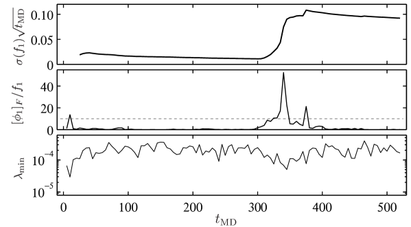
Figure 4: Normalized ${[\phi_{1}]_{\rm F}}$ and smallest eigenvalue from one ”sick” replicum of run II. Evidently the spike in ${[\phi_{1}]_{\rm F}}$ is dominating the statistical error $\sigma(f_{1})$.

Even though in the limit of infinite statistics configurations carrying very small eigenvalues are given the correct weight, depending on the algorithm this might be badly approximated for a typical ensemble size. Similar arguments referring in particular to the HMC algorithm motivated the introduction of the Polynomial Hybrid Monte Carlo (PHMC) algorithm in refs. [?].

Hence the difficulty in measuring fermionic correlation functions might be an efficiency problem related to the choice of the algorithm. To check this conjecture we employ a second algorithm and compare ensembles generated by HMC (with two pseudo–fermion fields) with PHMC ensembles. Indeed, PHMC can be tuned in such a way that it enhances the occurrence of configurations carrying small eigenvalues, thus resulting in a better sampling of this region of configuration space. A reweighting step is introduced to render the algorithm exact. As a preparation for the following discussions we want to recall some properties and introduce the notations concerning the PHMC.

2.2.1 The PHMC algorithm

One of the main ideas of the PHMC algorithm is to deliberately move away from importance sampling by using an approximation to the fermionic part of the lattice QCD action. More precisely, in an HMC algorithm the inverse of $\hat{Q}^{2}$ is replaced by a polynomial $P_{n,\epsilon}(\hat{Q}^{2})$ of degree $n$. Here $P_{n,\epsilon}(x)$ approximates $1/x$ in the range $\epsilon\leq x\leq 1$. As a consequence this algorithm stochastically implements the weight ${\rm d}U\det P^{-1}_{n,\epsilon}(\hat{Q}^{2})e^{-S_{g}}$, whereas standard HMC generates ensembles according to ${\rm d}U\det\hat{Q}^{2}e^{-S_{g}}$ with $S_{g}$ being the gauge part of the action and $U$ the gauge link configuration. Denoting averages over the PHMC ensemble by $\langle\dots\rangle_{\rm P}$, the correct sample average of an observable $\langle O\rangle$ can then be written as

$$\langle{O}\rangle=\langle O\omega\rangle_{\rm P}\;,\textrm{ where}\ \ \omega=\frac{W}{\langle W\rangle_{P}}\;,$$ (2.2)

and we introduce the reweighting factor $W$ as a (partially) stochastic estimate of $\det\{\hat{Q}^{2}P_{n,\epsilon}(\hat{Q}^{2})\}$. When using Chebyshev polynomials the relative approximation error for $\epsilon\leq x\leq 1$ is bounded by $\delta\simeq 2\exp(-2\sqrt{\epsilon}n)$.

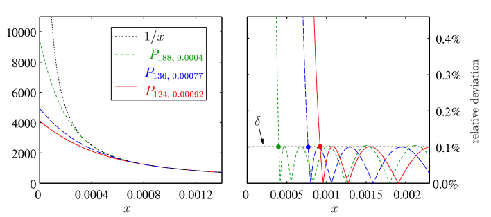
Figure 5: Three different Chebyshev polynomials approximating $1/x$, all with $\delta=0.001$. The right–hand plot shows the relative deviation from $1/x$ as a function of $x$. There the points $(\epsilon,\delta)$ are marked by dots.

To give an impression of the rôle of $\epsilon$ and $\delta$ we plot in Fig. 5 a set of polynomials $P_{n,\epsilon}(x)$ for typical (in our simulations) values of these parameters and compare them with $1/x$ in the region of small $x$. Depending on the smallest eigenvalue of $\hat{Q}^{2}$ the parameters $\epsilon$ and $n$ have to be tuned such that the reweighting factor does not fluctuate too much. The authors of ref. [?] suggested to take $\epsilon$ of the same order as $\langle\lambda_{\rm min}\rangle$ and in practice used $\epsilon\simeq 2\langle\lambda_{\rm min}\rangle$ and $\delta\lesssim 0.01$.

Recalling that PHMC replaces $\det\hat{Q}^{2}$ in the HMC weight with $\det P^{-1}_{n,\epsilon}(\hat{Q}^{2})$ and observing from Fig. 5 that $P_{n,\epsilon}(x)$ is smaller than $1/x$ for $x\leq\epsilon$, the aforementioned property of enhancing the occurrence of small eigenvalues is evident. At this point we would like to note that the fermionic contribution to the driving force in the PHMC is bounded from above since $P_{n,\epsilon}(x)$ is finite even at $x=0$. In this way the polynomial provides a regularized inversion of $\hat{Q}^{2}$, thus also addressing the problems mentioned in Section 2.1.

2.2.2 HMC vs. PHMC

Coming back to the comparison of samples from HMC and PHMC, we repeated run II with PHMC using a polynomial of degree $140$ and $\epsilon=6\cdot\!10^{-4}$, resulting in $\delta\simeq 0.002$. The ratio $\epsilon/\langle\lambda_{\rm min}\rangle$ turned out to be around $2.7$. In Fig. 6 we plot for this run the MC history of ${[\phi_{1}]_{\rm F}}$ and of ${[\phi_{1}]_{\rm F}}\cdot\omega$, which enters into eq. (2.2) if we consider $O={[\phi_{1}]_{\rm F}}$, i.e.

$$f_{1}=\langle{[\phi_{1}]_{\rm F}}\rangle=\langle{[\phi_{1}]_{\rm F}}\cdot\omega\rangle_{P}=\frac{\langle{[\phi_{1}]_{\rm F}}\cdot W\rangle_{P}}{\langle W\rangle_{P}}\;.$$ (2.3)

We first observe that apart from removing the largest spikes the inclusion of the reweighting factor does not seem to significantly change the relative fluctuations. This means that the parameters of the polynomial have been chosen properly. Events where ${[\phi_{1}]_{\rm F}}$ assumes a value ${\rm O}(10)$ times larger than $f_{1}$ are no longer isolated as in Fig. 3 but happen frequently, which means that the PHMC algorithm can more easily explore the associated regions in configuration space. This is what allows a reliable error estimate as shown in the upper part of Fig. 6, i.e. with 16 replica the asymptotic behavior of the error sets in after $t_{\rm MD}\!\simeq\!100$.

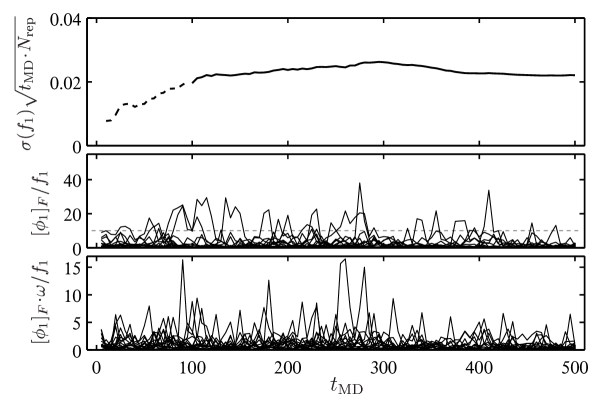
Figure 6: Monte Carlo history for the 16 replica of run III showing the correlation function ${[\phi_{1}]_{\rm F}}$ and the product ${[\phi_{1}]_{\rm F}}\cdot\omega$, where $\omega$ is the normalized reweighting factor. Our error estimate of $f_{1}$ shows the expected scaling behavior as soon as the run is long enough for a reliable extraction of $\tau_{\rm int}$.

The advantage of using PHMC instead of HMC can be clearly seen by considering the spread of $\sigma(f_{1})\sqrt{t_{\rm MD}}$ among the replica. We analyzed this quantity in extensions of runs II and III. The result is shown in figure Fig. 7, where the shaded areas represent the range of values covered by the 16 replica as a function of the MD time. In the limit of infinite statistics all replica should converge to the same value, which need not be the same for the two algorithms because of reweighting and different autocorrelation times. We see that the spread for the HMC data is more than twice as large as for PHMC, i.e. the error on $f_{1}$ is significantly harder to estimate with HMC.

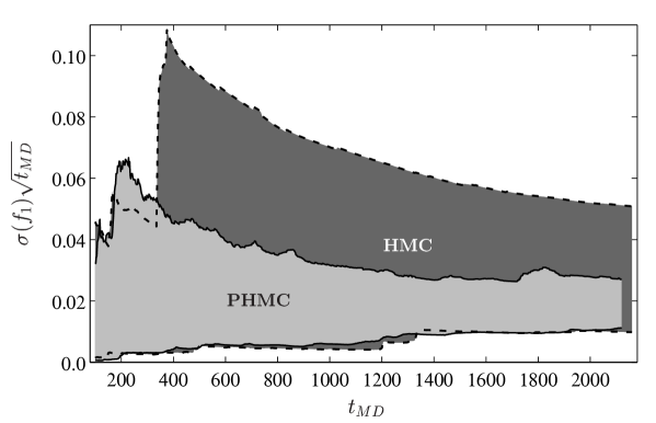
Figure 7: Monte Carlo history of $\sigma(f_{1})\sqrt{t_{\rm MD}}$ from extensions of runs II and III. For the two algorithms we show the ranges covered by the 16 replica.

What we are suggesting here is that the algorithm should be chosen depending on the type of observables and the parameter values. From our experience we conclude that PHMC sampling might just be more effective than HMC when computing fermionic quantities that are sensitive to small eigenvalues.

To gain some more insight into the difference in sampling we consider the distribution of $\lambda_{\rm min}$ since this is where we expect the largest effect. The distributions are analyzed by treating $\Lambda_{\rm bin}\!=\!\chi_{\rm bin}(\lambda_{\rm min})$ as a primary observable. Here $\chi_{\rm bin}$ denotes the characteristic function of each given bin in the histogram. We then perform our normal error analysis for $\langle\Lambda_{\rm bin}\rangle$, where eq. (2.2) has to be used if it is a PHMC sample. For comparison $\langle\Lambda_{\rm bin}\rangle_{\rm P}$ is also analyzed in this case.

The histograms in the upper part of Fig. 8 compare the results from 200 independent measurements produced by HMC and PHMC (runs II and III, respectively). As expected the distributions agree within errors. For the PHMC run we also plot the unreweighted histogram, i.e. $\langle\Lambda_{\rm bin}\rangle_{\rm P}$. Here we again confirm that with the parameters we chose for the polynomial the PHMC produces more configurations with small eigenvalues than HMC. As a consequence of the reweighting the errors at the infrared end of the spectrum should be smaller for the PHMC data. This is explicitly verified in the lower part of the plot where we show the ratio of the errors on $\langle\Lambda_{\rm bin}\rangle$ from the two algorithms. The three symbols refer to different bin sizes. The advantage in using PHMC to sample this part of the spectrum is significant and we will make use of this in the following discussion.

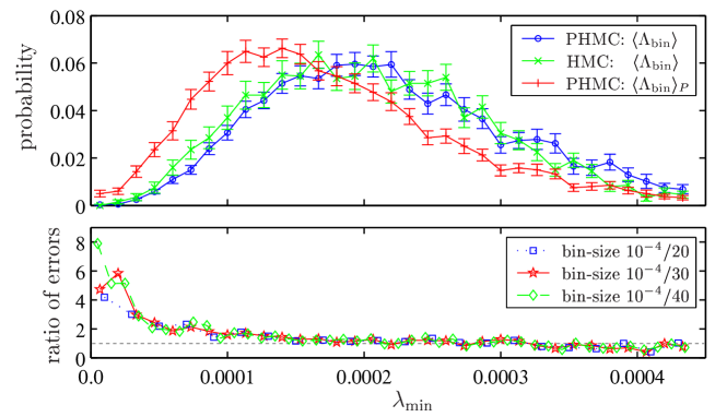
Figure 8: Upper panel: histograms of $\lambda_{\rm min}$, i.e. $\langle\Lambda_{\rm bin}\rangle$ vs. ’bin’, from runs II and III. For run III we also show $\langle\Lambda_{\rm bin}\rangle_{P}$. Lower panel (from the same data): ratio of the error on $\langle\Lambda_{\rm bin}\rangle$ from HMC to that from PHMC.

3 Comparison to the quenched case

In the previous section we studied various problems related to the occurrence of small eigenvalues. All the data presented there were produced at bare parameter values, which correspond to relatively large quark masses and small volumes. These small eigenvalues might therefore have a different nature from the ”physical” ones expected to show up in large volumes and/or close to the chiral limit. Here and in the next section we will establish them as cutoff–effects.

To this end we made an additional simulation at the parameters of run II and calculated the ten lowest–lying eigenvalues $\lambda_{i}$, $i=1\ldots 10$. In Fig. 9 the smallest eigenvalue, $\lambda_{1}$, is denoted by an open symbol. It seems that while $\lambda_{2}$ through $\lambda_{10}$ form a rather compact band, the lowest eigenvalue fluctuates to very small values quite independently of the others. It is expected and has been shown numerically [?] that the spectrum of the Dirac operator depends quite strongly on the bare gauge coupling. A well–defined lower bound should be recovered close to the continuum limit only. Therefore we take the strong fluctuations of $\lambda_{\rm min}$ as an indication for the presence of large cutoff–effects. Here we should point out that the eigenvalues of the Dirac operator are not on–shell quantities. Hence the Symanzik improvement programme does not necessarily reduce cutoff–effects here. Quenched experience even suggests that the opposite might be true [?].

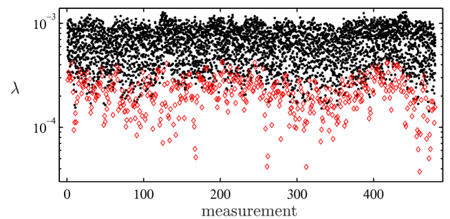
Figure 9: Monte Carlo history of the ten lowest eigenvalues at the parameters of run II. The open symbols denote $\lambda_{\rm min}$.

The occurrence of small eigenvalues at these bare parameters poses a somewhat unexpected problem in dynamical simulations. Comparing the quenched situation to the $N_{f}\!=\!2$ dynamical case, the naïve expectation is that at fixed bare parameters the probability of finding configurations with small eigenvalues should be reduced by the determinant. To us the more relevant question seems to be whether small eigenvalues are suppressed in a situation where the physical parameters (e.g. volume and pseudo–scalar mass) are kept constant.

Using the quenched data from ref. [?] and the dynamical data from refs. [?] and [?] (where an estimate of $r_{0}/a\!=\!5.21(6)$ for $\beta\!=\!5.2$ can be found) we chose the parameters of the quenched run V such that the lattice spacing and the (large volume) pseudo–scalar mass are matched to run IV. This was found to occur at almost equal bare current quark mass (see $Lm$ in Table 1). In Fig. 10 we compare the distributions of $\lambda_{\rm min}$ for these two runs. Two comments are in order here:

• For the dynamical run the mean value is shifted up from $1.44(1)\!\cdot\!10^{-4}$ to $1.72(5)\!\cdot\!10^{-4}$. This agrees with the naïve expectation but in a physically matched comparison it is a non–trivial observation.

• The distribution itself is significantly broader compared to the quenched case and in particular it is falling off more slowly towards zero. This means that even though $\langle\lambda_{\rm min}\rangle$ is larger for $N_{f}\!=\!2$ the probability of finding very small eigenvalues is enhanced.

The second point, i.e. that the lower bound of $\lambda_{\rm min}$ is less well–defined, seems to imply that at a lattice spacing of $a\approx 0.1\,{\rm fm}$ the cutoff–effects are much larger in the $N_{f}\!=\!2$ case. To substantiate this we will compare the distribution of $\lambda_{\rm min}$ to that from a run at finer lattice spacing and matched physical parameters.

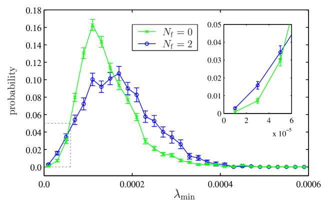
Figure 10: The histograms of $\lambda_{\rm min}$ from run IV ($N_{f}\!=\!2$) and run V ($N_{f}\!=\!0$). Despite its higher mean value the dynamical data show a much larger probability of finding very small eigenvalues.

4 Finer lattices

Apart from cutoff–effects, in the massless theory the Schrödinger functional coupling $\bar{g}^{2}$ is a function of the box size $L$ only [?,?]. We measured it on a small lattice of extension $L/a\!=\!4$ at $\beta=5.2$, obtaining a value of $\bar{g}^{2}\!=\!3.7(1)$. We then extrapolated to this value the $L/a\!=\!6$ data used in ref. [?] as a function of $\beta$. Our result from the matching is that for the two–flavor theory a bare gauge coupling of $\beta\!=\!5.5$ roughly corresponds to a lattice spacing, which is 1.5 times smaller than at $\beta\!=\!5.2$.

Hoping that the algorithmic difficulties arising from cutoff–effects would be much smaller in this situation, we simulated a $12^{3}\!\times\!27$ lattice at this value of $\beta$ (run VI) using the HMC algorithm. With the $\kappa$ we chose (and ignoring the change in renormalization factors) the bare quark mass $Lm$ is roughly matched to the heavier runs at $\beta\!=\!5.2$. We therefore compare run VI with run III.

Normally, a constant acceptance requires a decrease of the MD integration step–size if ones goes to finer lattices at fixed physical conditions. This argument is based on the scaling of the small eigenvalues, which influence the MD driving force. We found that $\langle\lambda_{\rm min}\rangle$ in run VI is a factor two smaller than in run III. Nevertheless, at $\beta\!=\!5.5$ the step–size necessary for a certain ($\simeq 90\%$) acceptance is roughly the same as at $\beta\!=\!5.2$. This indicates that the value of $\delta\tau$ we had to use in the HMC runs at $\beta\!=\!5.2$ was dictated by the occurrence of extremely small eigenvalues rather than by the average smallest eigenvalue. In addition, where in run I at the same average acceptance a maximum of $47$ proposals were rejected in a row, the maximum for run VI is $4$ trajectories. For this reason $e^{-\Delta H}$ shows no autocorrelation and its distribution is well separated from zero.

Concerning fermionic observables, we have not observed spikes and hence expect the error to scale properly. However, for an accurate estimate of the error on e.g. $f_{1}$ our present statistics is not yet sufficient.

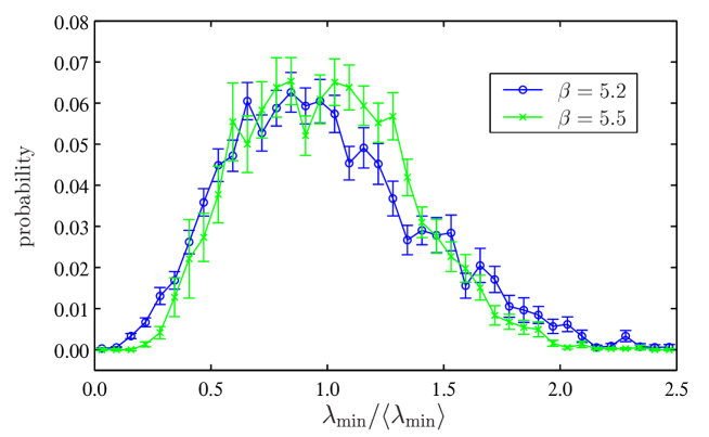
Figure 11: Normalized distributions of $\lambda_{\rm min}$ from runs III ($\beta\!=\!5.2$) and VI ($\beta\!=\!5.5$). While the data from the coarse lattice stretch almost to zero, the $\beta\!=\!5.5$ data seem to have a more well–defined lower bound.

The reason for these effects is the change in the distribution of $\lambda_{\rm min}$. To compensate for the different lattice spacing, Fig. 11 compares $\lambda_{\rm min}/\langle\lambda_{\rm min}\rangle$ from runs III and VI. One can clearly see that at the finer lattice spacing the probability of finding a smallest eigenvalue less than half its average is greatly reduced compared to $\beta\!=\!5.2$. The width of the distribution is smaller in this case and in particular the spectrum is now clearly separated from zero. Quantitatively, the normalized variance of $\lambda_{\rm min}$ is reduced from $0.18(1)$ to $0.13(2)$.

This comparison explicitly shows that the long tail of the eigenvalue distribution we observed at $a\simeq 0.1\,{\rm fm}$, and which caused the problems we have discussed, is a cutoff-effect. Matching also run VI to a quenched simulation (run VII), we again found an upward shift of $\langle\lambda_{\rm min}\rangle$ for the dynamical case. In addition, at this finer lattice spacing, the tails of the distributions of $\lambda_{\rm min}$ look already very similar to each other as shown in Fig. 12.

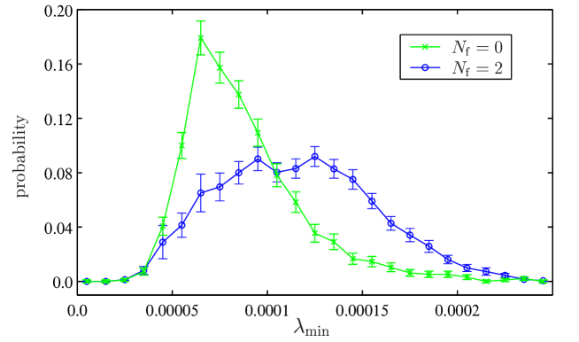
Figure 12: The histograms of $\lambda_{\rm min}$ from run VI ($N_{f}\!=\!2$) and run VII ($N_{f}\!=\!0$). At this finer lattice spacing the lower end of the spectrum appears to be similar in the quenched and the dynamical case.

5 Conclusions

At a lattice cutoff of approximately $2\;\rm{GeV}$ we have studied the behavior and performance of HMC–type algorithms in an intermediate size volume of $1\,{\rm fm}^{4}$. We discussed problems related to the occurrence of small eigenvalues in two–flavor dynamical simulations with improved Wilson fermions. We found these small eigenvalues to be responsible for large Hamiltonian violations in the molecular dynamics. Even for integration step–sizes such that the acceptance is $80\sim 90\%$ those can still cause long periods of rejection, thus degrading algorithmic performance. However, in spite of employing only single–precision arithmetics we never observed reversibility violations.

In addition, those eigenvalues make the estimate of fermionic quantities very difficult. The naïve intuition is that the fermionic determinant should suppress small eigenvalues compared to the quenched case. Through a direct comparison at matched physical parameters we indeed verified that $\langle\lambda_{\rm min}\rangle$ is larger with two dynamical flavors. On the other hand there is no obvious expectation for the tail of the distribution and we observed that it extends further towards zero than in the quenched case. Given the infrared cutoff induced by the Schrödinger functional boundary conditions and the quark mass we interpret this as a lattice artifact. We were able to confirm this picture with a simulation at finer lattice spacing, where the spectrum turned out to have a much sharper lower bound.

In our study we found that the PHMC algorithm is more efficient than HMC (with two pseudo–fermions) in incorporating the contribution to the path integral of configurations carrying small eigenvalues. In other words, the distortion of the spectrum by cutoff–effects actually makes it advantageous to deviate from importance sampling. Also without such special problems we found PHMC at least comparable in performance to HMC (in our implementations).

We want to emphasize that the problems discussed here do not occur only in the Schrödinger functional setup. Without this infrared regulator they are expected to show up already at larger quark masses.

Acknowledgements. We are grateful to R. Sommer for discussions and a critical reading of the manuscript. Discussions with S. Aoki, S. Hashimoto and T. Kaneko are also acknowledged. We thank NIC/DESY Zeuthen for allocating computer time on the APEmille machines indispensable to this project and the APE group for their professional and constant support. This work is supported in part by the Deutsche Forschungsgemeinschaft in the SFB/TR 09-03, “Computational Particle Physics” and the Graduiertenkolleg GK271.

References

- [1] S. Aoki et al. [JLQCD Collaboration], Nucl. Phys. Proc. Suppl. 106 (2002) 263.
- [2] R. Sommer et al. [ALPHA Collaboration], Nucl. Phys. Proc. Suppl. 129-130 (2004) 405.
- [3] J. Heitger [ALPHA Collaboration], Nucl. Phys. B 557 (1999) 309.
- [4] R. Hoffmann et al. [ALPHA Collaboration], Nucl. Phys. Proc. Suppl. 129-130 (2004) 423.
- [5] S. Dürr and M. Della Morte, Nucl. Phys. Proc. Suppl. 129-130 (2004) 417.
- [6] P. de Forcrand and T. Takaishi, Nucl. Phys. Proc. Suppl. 53 (1997) 968.
-
[7]
R. Frezzotti and K. Jansen,
Phys. Lett. B 402 (1997) 328.
R. Frezzotti and K. Jansen, Nucl. Phys. B 555 (1999) 395.
R. Frezzotti and K. Jansen, Nucl. Phys. B 555 (1999) 432. - [8] M. Lüscher, R. Narayanan, P. Weisz and U. Wolff, Nucl. Phys. B 384 (1992) 168.
- [9] S. Sint, Nucl. Phys. B 421 (1994) 135.
- [10] M. Lüscher, S. Sint, R. Sommer and P. Weisz, Nucl. Phys. B 478 (1996) 365.
- [11] M. Lüscher et al. [ALPHA Collaboration], Nucl. Phys. B 491 (1997) 323.
- [12] K. Jansen and R. Sommer [ALPHA Collaboration], Nucl. Phys. B 530 (1998) 185 [Erratum-ibid. B 643 (2002) 517].
- [13] N. Yamada et al. [JLQCD Collaboration], hep-lat/0406028.
- [14] A. Bode, P. Weisz and U. Wolff [ALPHA Collaboration], Nucl. Phys. B 576 (2000) 517 [Erratum-ibid. B 600 (2001) 453 and B 608 (2001) 481].
- [15] S. Sint and P. Weisz, Nucl. Phys. B 502 (1997) 251.
- [16] M. Lüscher and P. Weisz, Nucl. Phys. B 479 (1996) 429.
-
[17]
M. Hasenbusch,
Phys. Lett. B 519 (2001) 177.
M. Hasenbusch and K. Jansen, Nucl. Phys. B 659 (2003) 299. - [18] M. Della Morte et al. [ALPHA Collaboration], Comput. Phys. Commun. 156 (2003) 62.
- [19] S. Capitani, M. Lüscher, R. Sommer and H. Wittig [ALPHA Collaboration], Nucl. Phys. B 544 (1999) 669.
- [20] B. Joo et al. [UKQCD Collaboration], Phys. Rev. D 62 (2000) 114501.
- [21] U. Wolff [ALPHA Collaboration], Comput. Phys. Commun. 156 (2004) 143.
-
[22]
Y. Namekawa et al. [CP-PACS Collaboration],
Nucl. Phys. Proc. Suppl. 119 (2003) 335.
Y. Namekawa et al. [CP-PACS Collaboration], hep-lat/0404014. - [23] C. R. Allton et al. [UKQCD Collaboration], hep-lat/0403007.
- [24] R. Frezzotti, Nucl. Phys. Proc. Suppl. 119 (2003) 140.
- [25] P. Hernandez, K. Jansen and M. Lüscher, Nucl. Phys. B 552 (1999) 363.
- [26] T. DeGrand, A. Hasenfratz and T. G. Kovacs, Nucl. Phys. B 547 (1999) 259.
- [27] J. Garden, J. Heitger, R. Sommer and H. Wittig [ALPHA Collaboration], Nucl. Phys. B 571 (2000) 237.
- [28] S. Aoki et al. [JLQCD Collaboration], Phys. Rev. D 68 (2003) 054502.
- [29] C. R. Allton et al. [UKQCD Collaboration], Phys. Rev. D 65, 054502 (2002).
- [30] A. Bode et al. [ALPHA Collaboration], Phys. Lett. B 515, 49 (2001). M. Della Morte et al. [ALPHA Collaboration], Nucl. Phys. Proc. Suppl. 119 (2003) 439.