Abstract

The inclusion of electromagnetic effects in unquenched QCD can be accomplished using ensembles generated in dynamical simulations with pure QCD provided the change in the quark determinant induced by a weak electromagnetic field can be efficiently computed. A stochastic technique for achieving this in the case of dynamical domain wall calculations is described.

1 Introduction

Previous work in quenched QCD [1, 2] has established the possibility of computing quark masses including electromagnetic effects, as well as fine structure of hadron multiplets, by explicitly coupling the quark fields to a weak electromagnetic U(1) gauge field superimposed on pure QCD gauge fields generated in a conventional Monte Carlo simulation. Although the pattern of fine structure revealed in these quenched calculations qualitatively matches the experimental splittings for the meson and baryon octets, a credible quantitative computation clearly requires a fully unquenched treatment of both the gluon and photon dynamics. In this paper we present a technique for including electromagnetic effects in preexisting ensembles of pure QCD gaugefields generated with dynamical domain wall quarks. Although we describe the method for domain wall quarks (preferred in this case for the enhanced chiral symmetry and control over quark mass renormalization available in this formulation), the technique applies just as well to other fermion discretizations such as Wilson quarks (with or without clover improvement).

To illustrate the basic idea, we note that the path integral for quarks coupled to both SU(3) gluons (represented by conventional compact link variables $U$, with action $S_{\rm gl}$) and an abelian photon field $A$ (with a noncompact action $S_{\rm em}(A)=\frac{1}{4e^{2}}\sum_{n\mu\nu}(\nabla_{\mu}A_{n\nu}-\nabla_{\nu}A_{n\mu})^{2}$,[1], in Coulomb gauge) can be written (somewhat schematically):

$$Z_{SU(3){\rm x}U(1)} = \int{\cal D}U{\cal D}A\;\;{\rm det}(M(U,A))e^{-S_{\rm gl}(U)-S_{\rm em}(A)}$$ (1)

$$= \int{\cal D}U\;\;{\rm det}(M(U,A=0))e^{-S_{\rm gl}(U)}\int{\cal D}A\frac{{\rm det}(M(U,A))}{{\rm det}(M(U,A=0))}e^{-S_{\rm em}(A)}$$ (2)

where $M(U,A)$ is the matrix defining the lattice quark action in the presence of the SU(3) field $U$ together with the abelian photon field $A$. Evidently, at least in principle, the simulation of physical observables in the presence of both QCD and electromagnetism can be effected by superimposing photon fields generated with weight $e^{-S_{\rm em}(A)+\ln{\frac{{\rm det}(M(U,A))}{{\rm det}(M(U,0))}}}$ on a pre-existing ensemble $U$ generated by a pure SU(3) dynamical QCD simulation. This approach will of course only be feasible provided:

1. The variance of the determinant ratios $\ln{(\frac{{\rm det}(M(U,A))}{{\rm det}(M(U,0))})}$ is tolerably small, and

2. there is a reasonably efficient strategy for computing the above determinant ratios for a given gluon field $U$ and a suitable ensemble of weak photon fields $A$.

Given the extremely expensive nature of full dynamical QCD calculations, especially in chirally invariant formulations such as with domain wall or overlap fermions, it is unrealistic to expect that dynamical configurations with explicitly simulated photon fields, at a variety of quark masses and electric charges, will be available in the foreseeable future. Consequently, a procedure which allows us to exploit dynamical configurations generated for electrically neutral quarks to study issues of electromagnetic fine structure would clearly be very useful.

In Section 2, we show how the determinant ratios appearing in (2) may be computed exactly, at least for small lattices, for the domain wall formulation of SU(3)xU(1) gauge theory, using a Lanczos algorithm. Although this approach is not feasible for large lattices, it gives an exact result on smaller lattices which is extremely useful in checking the correctness and accuracy of the stochastic approach to computing determinant ratios described in Section 3. In Section 4 we give further details regarding the computational effort required to extract determinant ratios at a given level of accuracy.

2 Exact Computation of Domain Wall Determinants

In the domain wall formulation [3, 4] of lattice quark fields, the matrix $D(U)$ defining the quadratic form for the fermionic action can be rendered hermitian by premultiplication with the four-dimensional $\gamma_{5}$ matrix and the time inversion operator $R$ in the fifth dimension (assumed of extent $L_{5}$ henceforth), yielding a matrix $M(U)\equiv R\gamma_{5}D(U)$ which as an $L_{5}$x$L_{5}$ dimensional block matrix takes the form (for ease of display, taking $L_{5}$=6)

$$M=\left(\begin{array}[]{cccccc}-m_{q}P_{+}&0&0&0&-P_{-}&a_{5}H-\gamma_{5}\\ 0&0&0&-P_{-}&a_{5}H-\gamma_{5}&P_{+}\\ 0&0&-P_{-}&a_{5}H-\gamma_{5}&P_{+}&0\\ 0&-P_{-}&a_{5}H-\gamma_{5}&P_{+}&0&0\\ -P_{-}&a_{5}H-\gamma_{5}&P_{+}&0&0&0\\ a_{5}H-\gamma_{5}&P_{+}&0&0&0&m_{q}P_{-}\end{array}\right)$$

where $P_{\pm}\equiv\frac{1}{2}(1\pm\gamma_{5})$, $m_{q}$ is the bare quark mass, $a_{5}$ the lattice spacing in the fifth dimension, $H$ the four-dimensional hermitian Wilson operator with an appropriately chosen domain wall mass (or hopping parameter $\kappa$). It is easy to establish the following trace identities

$${\rm Tr}(M) = 0$$ (3)

$${\rm Tr}(M^{2}) = 12V(L_{5}(1-\frac{a_{5}}{2\kappa})^{2}+L_{5}(1+4a_{5}^{2})+m_{q}^{2}-1)$$ (4)

where $V$ is the volume of the four-dimensional lattice. These trace identities serve as useful checks on the accuracy of the computed spectrum of $M$: identities involving higher powers of $M$ can also be derived, involving plaquette (or even higher loop) sums, but will not be needed here. Of course, ${\rm det}(M)={\rm det}(D)$.

For not too large lattices, the Lanczos algorithm can be used to extract the complete spectrum of the hermitian matrix $M$: for a review of the issues involved in computing complete spectra with Lanczos, we refer the reader to [5]. In this paper we shall consider 5-dimensional lattices dimensioned $L^{4}$x$L_{5}$ with $L=$4,6 and $L_{5}$=12. For the case $L=$4, the matrix $M$ has dimension 12$VL_{5}$=36864, and resolving the complete spectrum to 9 significant figures requires on the order of 200,000 Lanczos sweeps. One then finds that ${\rm Tr}(M)\simeq$10^-9 and the left and right hand sides of (4) agree to 9 significant figures. The computational effort required grows as the square of the dimension of $M$, however, and on larger lattices one eventually encounters missed eigenvalues (due to accidental close degeneracies) which make this brute-force approach to extracting a full spectrum, and determinant, ultimately impractical. However, having an “exact” result for the domain-wall determinant (at least, to 9 significant figures) will turn out to be a useful check on the accuracy of the stochastic methods described below.

3 Stochastic Procedure for Determinant Ratios

The stochastic formalism developed by Golub and coworkers [6] provides an approach to the calculation of determinant ratios which allows us to go to larger, and more physically realistic lattices. This technique was first applied to the quark determinant problem in lattice QCD by Irving and Sexton [7]. In this approach, given a positive definite hermitian matrix $P$, the close connection between Lanczos recursion and Gaussian integration is exploited to compute an arbitrary diagonal matrix element $<v|f(P)|v>$ of any differentiable function $f(P)$ of the matrix $P$. Any such matrix element can be written as a spectral sum which can then be interpreted as a Riemann-Stieltjes integral computable via the usual variety of Gaussian quadrature rules (Gauss, Gauss-Radau, Gauss-Lobatto, etc.). It turns out that the appropriate weights for the Gaussian quadrature are directly related to the spectrum of the tridiagonal matrix generated by Lanczos recursion on $P$ (for further details, see [6]). With a technique for computing diagonal matrix elements in hand, this approach then leads immediately to a stochastic method for unbiased estimates of the ${\rm Tr}(f(P))$ as the average over an ensemble of diagonal expectations of $f(P)$ with respect to a set of random vectors $|z_{i}>$ where each vector has components $\pm 1$ chosen at random:

$${\rm Tr}(f(P)) = E(<z|f(P)|z>)$$ (5)

$$var(<z|f(P)|z>) = 2\sum_{i\neq j}|f(P)_{ij}|^{2}$$ (6)

The above method can be fruitfully applied to our problem- the evaluation of $\frac{{\rm det}(M(U,A))}{{\rm det}(M(U,0))}$- as follows. Choosing

$$P\equiv M(U,0)^{-1}M(U,A)^{2}M(U,0)^{-1}$$ (7)

we then have a positive definite hermitian matrix $P$ as required for the algorithm described above (for the work described in this paper, we have performed the required inversions of $M(U,0)$ using the minimum residual algorithm [8]). Choosing $f(P)=\ln{(P)}$, we obtain the (log of the square of the) desired determinant ratio. Moreover, for sufficiently weak electromagnetic fields $A$ it is clear that $P$ is close to the identity, which has the following salutary consequences:

1. As we shall see shortly, the Lanczos recursion to compute the individual diagonal matrix elements $<z|\ln{(P)}|z>$ converges extremely rapidly: in fact 4 or 5 Lanczos sweeps (corresponding to 8 or 10 inversions of the domain wall matrix $M$) are typically sufficient to obtain the matrix element to single precision accuracy.

2. As $P$ is close to the identity, (6) implies that the variance of the diagonal matrix elements should also be small, allowing us to obtain a good estimate of the trace with an ensemble of manageable size.

We have studied these issues on a variety of small lattices, generating pure SU(3) quenched configurations (at $\beta$=6.0) as the strong interaction background field, and Coulomb gauge photon field configurations corresponding to electric charge $e_{q}=-0.1$ (roughly, the down quark charge). On a 4⁴x12 lattice we then typically find $\ln{\frac{{\rm det}(M(U,A))}{{\rm det}(M(U,0))}}=\frac{1}{2}{\rm Tr}\ln{(P)}\simeq-5$. For a specific diagonal element $<z|\ln{(P)}|z>$ with a typical random vector $|z>$, the convergence of the Lanczos estimates is indicated in Table 1, both for 4⁴x12 and for 6⁴x12 lattices. In either case, the convergence to seven or eight significant figures occurs after less than 10 Lanczos sweeps, with the rapidity of convergence basically insensitive to the lattice volume. The computational effort required for the Lanczos recursion is of course dominated by the inversions of the domain wall operator $M(U,0)$.

Table 1: Convergence of Lanczos estimates for a diagonal element of $\ln{(P)}$

Lanczos sweep	$<z|\ln{(P)}|z>,L=4$	$<z|\ln{(P)}|z>,L=6$
2	-11.29817352	-53.44524316
3	-11.54470058	-55.10595906
4	-11.54923739	-55.14478821
5	-11.54931955	-55.14572594
6	-11.54932110	-55.14575078
7	-11.54932113	-55.14575146
8	-11.54932113	-55.14575148

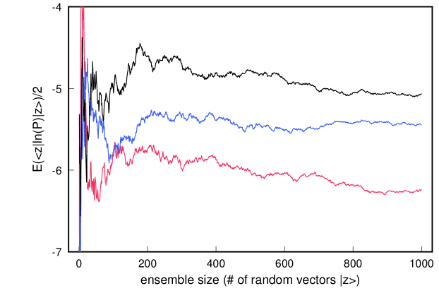
Figure 1: Ensemble convergence for log(determinant ratio),varying photon field, 4⁴x12

The computation of the determinant ratio, or equivalently the trace of $\ln{P}$, requires repeating the evaluation of the diagonal matrix element in a random vector $|z>$ many times, but this part of the procedure is of course trivially parallelizable as the random vectors (and resulting estimates of the trace) are completely independent. We show in Figure 1 the rate of convergence of the desired determinant ratio $E(<z|\ln{(P)}|z>)/2$ as a function of the ensemble size, up to a final sample size of 1000 random vectors, for three statistically independent photon field $A$ superimposed on the same background QCD field $U$. For the red curve, the exact (log)ratio of determinants, evaluated by computation of the complete spectrum as described in the preceding section, gives -6.1522, while the stochastic result (again, for 1000 random vectors) is -6.2384$\pm$0.1414. For the blue curve, the comparison is -5.3791 to -5.4472$\pm$0.1346, and for the black curve -5.0609 to -5.0635$\pm$0.1388. On a 4⁴x12 lattice, each evaluation of $<z|f(P)|z>$ in (5) takes about 20 seconds on a Xeon 2.8GHz PC. Note that the variation of the log determinant ratio is of order unity between different configurations. In Figure 2 the same convergence issues are displayed, this time varying both the abelian $A$ and nonabelian $U$ background fields.

Figure 2: Ensemble convergence for log(determinant ratio),varying photon,gluon fields, 4⁴x12

We have also repeated the stochastic determination of determinant ratios for a variety of 6⁴x12 lattices (with the same mass and coupling parameters as above), and Figure 3 shows the convergence from an ensemble of 4000 estimates for three different U(1) fields superimposed on a fixed QCD background. The variation of the log(determinant ratio) from one U(1) field to another again is of order unity. The total variance (6) turns out to be linear in the volume of the lattice: for $L$=4 we find a variance per site of 0.0063(2), while for $L$=6 the variance per site is 0.0066(5). The computed log(determinant ratio) is also of course an extensive quantity proportional to the lattice volume, so we conclude that we can achieve a fixed relative error in the log(determinant ratio) evaluation with a fixed ensemble size, or a fixed absolute error by increasing the number of stochastic estimates linearly with the lattice volume. Thus the absolute error on the log(determinant ratio) achieved for the 6⁴x12 lattices with 4000 estimates is about 0.16, comparable to the accuracy achieved with 1000 estimates on the smaller lattices (which are about one fifth the volume). As emphasized previously, the evaluations of $<z|f(P)|z>$ in (5) for different random vectors $|z>$ are completely independent so this average is trivially parallelizable with 100% efficiency.

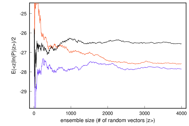
Figure 3: Ensemble convergence for log(determinant ratio),varying photon field, 6⁴x12

4 Computational Issues

We have described two different routes to computing the electromagnetic variation of the quark determinant in unquenched QCD with domain wall quarks: the direct, “brute force” evaluation of the complete spectrum of the (hermitian) domain wall operator via Lanczos recursion, or a stochastic, approximate evaluation using the Golub-Bai-Fahey method. The first approach, in which the Lanczos recursion is carried out in double precision, delivers a result for the determinant (provided all eigenvalues can be resolved) which is typically accurate to a precision 5 or 6 significant places short of double precision, with the loss of accuracy due to the need for distinguishing spurious from real eigenvalues [9]. The computational effort scales superficially as $V^{2}$ for lattice volume $V$ (where the first factor of volume arises from the multiplication by $M(U,A)$ at each Lanczos sweep, and the second from the fact that evaluation of the complete spectrum requires a number of Lanczos sweeps greater than and roughly proportional to $V$). However, for larger lattices the eigenvalue density rises to the point where double precision Lanczos recursions will be unable to resolve many of the eigenvalues, and the method simply becomes impractical in the absence of hardware-implemented extended precision arithmetic. Moreover, the most efficient techniques for diagonalization of the tridiagonal Lanczos matrix (e.g. the QL algorithm with implicit shifts [10]) are intrinsically serial by nature, which makes parallelization of this part of the procedure difficult (although less efficient parallel algorithms, based on the Sturm sequence property [11], have been used successfully for small lattices). The stochastic approach described in the previous section also scales as $V^{2}$ with the lattice volume, if we require a fixed absolute error in the log(determinant ratio), but does not require extended precision arithmetic as we go to larger lattices. Moreover, parallelization of this approach is trivial, as pointed out above. For the lattices studied here ($L$=4,6,$L_{5}$=12) the two methods are comparable in computational effort (if we require an error in the stochastic approach at the few percent level), so we conclude that the stochastic approach is probably the appropriate technique for larger systems.

5 Acknowledgements

The work of A. Duncan was supported in part by NSF grant 010487-NSF. A.D. is grateful for the hospitality of the Max Planck Institut für Physik (Werner Heisenberg Institut), where part of this work was done. The work of E. Eichten was performed at the Fermi national Accelerator Laboratory, which is operated by University Research Association, Inc., under contract DE-AC02-76CH03000.

References

- [1] A. Duncan, E. Eichten and H. Thacker, Phys. Rev. Lett. 76 (1996) 3894.
- [2] A. Duncan, E. Eichten and H. Thacker, Physics Letters B409 (1997) 387.
- [3] Y. Shamir, Phys. Rev. D59 (1999)054506.
- [4] A. Borici, hep-lat/0402035.
- [5] A. Duncan, E. Eichten, R. Roskies, and H. Thacker, Phys.Rev.D60 (1999)054505.
- [6] Z. Bai, M. Fahey and G. Golub, Stanford preprint SCCM95-09.
- [7] A.C. Irving and J. C. Sexton, Phys. Rev. D55 (1997)5456.
- [8] “Numerical Recipes in C”, W.H. Press et al, p. 85 (Cambridge University Press, 1992).
- [9] T. Kalkreuter, Comput.Phys.Commun. 95 (1996) 1.
- [10] “Numerical Recipes in C”, W.H. Press et al, p. 478 (Cambridge University Press, 1992).
- [11] “Matrix Computations”, G.H. Golub and C.F. van Loan, p.440 (johns Hopkins University Press 1996).