SHEP-0413

CPT-2004/P.024

DESY 04-090

${\rm SU(3)}$ lattice gauge theory with a mixed fundamental and adjoint plaquette action:
Lattice artefacts

M. Hasenbusch^a and S. Necco^b

^a Department of Physics and Astronomy, University of Southampton,

Southampton SO17 1BJ, United Kingdom

^b Centre de Physique Théorique

CNRS Luminy, Case 907 F-13288, Marseille Cedex 9, France

e-mail: hasenbus@phys.soton.ac.uk, necco@cpt.univ-mrs.fr

We study the four-dimensional ${\rm SU(3)}$ gauge model with a fundamental and an adjoint plaquette term in the action. We investigate whether corrections to scaling can be reduced by using a negative value of the adjoint coupling. To this end, we have studied the finite temperature phase transition, the static potential and the mass of the $0^{++}$ glueball. In order to compute these quantities we have implemented variance reduced estimators that have been proposed recently. Corrections to scaling are analysed in dimensionless combinations such as $T_{c}/\sqrt{\sigma}$ and $m_{0^{++}}/T_{c}$. We find that indeed the lattice artefacts in e.g. $m_{0^{++}}/T_{c}$ can be reduced considerably compared with the pure Wilson (fundamental) gauge action at the same lattice spacing.

1 Introduction

Due to the enormous effort required by lattice QCD simulations, one is restricted to rather coarse lattice spacings. Therefore it is important to choose the lattice action such that already at a coarse lattice spacing the lattice artefacts are small. In the past, various proposals had been made to this end.

One approach are so called perfect actions (for recent work on this subject see e.g. ref. [1]). Here one tries to avoid lattice artefacts completely, at the price of, in principle, an infinite number of terms in the action. In order to make this approach work practically, the set of terms has to be truncated to a finite, still large number of terms. The error introduced by this truncation is hard to estimate a priori.

Alternatively, Symanzik [2] has proposed a scheme that allows to eliminate lattice artefacts systematically, order by order in the lattice spacing and the coupling constant. For the SU(3) lattice gauge theory this has been worked out by Lüscher and Weisz [3] up to the 1-loop level in perturbation theory to eliminate $O(a^{2})$ corrections.

Since we work at rather large values of the gauge-coupling it is not clear a priori, whether the 1-loop improvement of ref. [3] is of any help. Only studies (see e.g. ref. [4]) of the scaling behaviour of various quantities can clarify this question.

Here, we pursue a rather ad hoc approach. It is well established that the pure SU(3) gauge theory in four dimensions has a line of first order phase transitions with an end-point at [5]

$$(\beta_{f},\beta_{a})=(4.00(7),2.06(8))\;\;\;.$$ (1)

For the precise definition of $\beta_{f}$ and $\beta_{a}$ see eq. (7) below. At such transitions, lattice artefacts might completely disguise the continuum physics. Here, in particular, the mass $m_{0^{++}}$ of the lightest glueball $0^{++}$ goes to zero as the end-point, eq. (1), is approached [6]. As a relic of this behaviour, the estimate of $m_{0^{++}}/T_{c}$ ($T_{c}$ is the location of the finite temperature phase transition) at $\beta_{a}=0$, for $5.5<\beta_{f}<6.0$ is much smaller than the continuum result. Here, we study whether the scaling behaviour can be improved by staying apart from the transition line by choosing negative values of $\beta_{a}$. Recently one of us [4] has studied gauge actions with $2\times 1$ - Wilson loops in addition to the plaquette. These actions are motivated by the RG-group and the Symanzik improvement programme. Indeed, for the so called Iwasaki action [7] an improved scaling behaviour was observed. Here we investigate whether by adding the adjoint part to the action similar benefits can be achieved, while keeping the action as local as possible; i.e. using plaquette terms only. For the mixed fundamental-adjoint action, it is straightforward to construct a transfer matrix along the lines of ref. [47]. However, for our choices of $\beta_{a}$, it is not positive. For a detailed discussion see the appendix.

An other important question (that we do not study here) is, whether dislocations, i.e. topological objects that are pure lattice artefacts, can be suppressed by a modification of the standard Wilson gauge action.

The outline of our paper is as follows: First we give the definition of the model and the observables that we have studied. Next we discuss the Monte Carlo algorithm that was used to generate the gauge-configurations. In section 4 we study the finite temperature phase transition. In section 5 we extract the string tension $\sigma$ from the Polyakov loop correlation function. To this end we have implemented a variant of the variance reducing algorithm proposed by Lüscher and Weisz [8]. Next, in section 6, we determine the mass $m_{0^{++}}$ of the lightest glueball $0^{++}$. Also here, we have employed a new algorithm [9], to reduce the variance of correlation functions. Based on these results, we compute the dimensionless quantities $T_{c}/\sqrt{\sigma}$ and $m_{0^{++}}/T_{c}$.

2 The model

We consider a hypercubical lattice with the linear extension $aN_{s}$ in the spacial directions and $aN_{t}$ in the temporal direction. $a$ is the lattice spacing. $N_{s}$ and $N_{t}$ are integer numbers. In all directions, periodic boundary conditions are applied.

The action describing the pure SU(N) lattice gauge theory containing plaquette terms only, can be written in the general form [10]

$$S\;=\;\sum_{\alpha}\tilde{\beta_{\alpha}}\;\sum_{P}\left[1-\frac{1}{d(\alpha)}\mbox{Re}\mbox{Tr}_{\alpha}U_{P}\right]\;\;,$$ (2)

where the sum over $\alpha$ indicates the sum over all representations of SU(N), $\tilde{\beta_{\alpha}}$ is the coupling associated with each representation, $d(\alpha)$ is the dimension of the representation, $\mbox{Tr}_{\alpha}$ is the trace in the given representation and $U_{P}$ is the path ordered product of the link variables along an elementary plaquette $P$:

$$U_{P}(x,\mu,\nu)=U_{x,\mu}U_{x+\hat{\mu},\nu}U_{x+\hat{\nu},\mu}^{{\dagger}}U_{x,\nu}^{{\dagger}}\;\;,$$ (3)

where $x$ labels the sites of the lattice and $\hat{\mu}$ is a unit vector in the $\mu$-direction.

In particular, we will consider the mixed fundamental-adjoint action

$$S\;=\;\tilde{\beta_{f}}\;\sum_{P}\left[1-\frac{1}{N}\mbox{Re}\mbox{Tr}_{f}U_{P}\right]+\tilde{\beta_{a}}\;\sum_{P}\left[1-\frac{1}{N^{2}-1}\mbox{Re}\mbox{Tr}_{a}U_{P}\right]\;\;.$$ (4)

Using the identity

$$\mbox{Tr}_{a}U=\mbox{Tr}_{f}U^{{\dagger}}\mbox{Tr}_{f}U\;-\;1$$ (5)

and defining

$$\beta_{f}=\tilde{\beta_{f}},\quad\beta_{a}=\frac{N^{2}}{N^{2}-1}\tilde{\beta_{a}}\;\;,$$ (6)

one obtains

$$S\;=\;\beta_{f}\;\sum_{P}\left[1-\frac{1}{N}\mbox{Re}\mbox{Tr}_{f}U_{P}\right]\;+\;\beta_{a}\;\sum_{P}\left[1-\frac{1}{N^{2}}\mbox{Tr}_{f}U_{P}^{{\dagger}}\mbox{Tr}_{f}U_{P}\right]\;\;,$$ (7)

which is the form that we will use in the following for SU(3). In the naive continuum limit the bare coupling $g_{0}$ for the action eq. (7) is given by

$$\frac{6}{g_{0}^{2}}=\beta_{W}=\beta_{f}+2\beta_{a}\;\;,$$ (8)

where we have introduced, following the literature, the notion of an “equivalent Wilson coupling” $\beta_{W}$.

2.1 Observables

In the following we define the basic observables that we have studied. The fundamental plaquette is given by

$$E_{f}=\frac{1}{6V}\sum_{x,\mu,\nu>\mu}\langle\mbox{Tr}_{f}U_{P}\rangle\;\;,$$ (9)

where $V=N_{s}^{3}N_{t}$ is the number of points of the lattice.
The adjoint plaquette can be defined by

$$E_{a}=\frac{1}{18V}\sum_{x,\mu,\nu>\mu}\langle\mbox{Tr}_{f}U^{\dagger}_{P}\mbox{Tr}_{f}U_{P}\rangle\;\;.$$ (10)

To study the finite temperature phase transition and the potential of static quarks we consider the Polyakov loop

$$P_{\vec{x}}=\mbox{Tr}_{f}\prod_{t}U_{\vec{x},t,0}\;\;,$$ (11)

where $U_{\vec{x},t,\mu}$ is the link variable starting in $\vec{x},t$ in the direction $\mu$. In particular, we study the histogram associated with the quantity

$$\Omega=\frac{1}{N_{s}^{3}}\sum_{\vec{x}}P_{\vec{x}}\;\;.$$ (12)

3 Simulation algorithm

We have simulated the model with a local Metropolis procedure. The proposal for a new value of a link variable is generated by a Cabbibo-Marinari (CM) heat-bath update [11] of a single SU(2)-subgroup for the action

$$S_{0}\;=\;\beta_{f}^{\prime}\;\sum_{P}\left[1-\frac{1}{N}\mbox{Re}\mbox{Tr}_{f}U_{P}\right]\;\;.$$ (13)

This proposal is then accepted with the probability

$$A=\mbox{min}\left[1,\exp(-S(U^{\prime})+S_{0}(U^{\prime})+S(U)-S_{0}(U))\right]\;\;,$$ (14)

where $U$ is the original gauge field and $U^{\prime}$ is the proposal. $\beta_{f}^{\prime}<\beta_{f}$ is tuned such that the optimal acceptance rate is obtained. In addition, we have performed overrelaxation (OV) updates [12] that keep the fundamental part of the action constant. Here, we accepted the proposal with the probability

$$A=\mbox{min}\left[1,\exp(-S_{a}(U^{\prime})+S_{a}(U))\right]\;\;,$$ (15)

where

$$S_{a}(U)=\;\beta_{a}\;\sum_{P}\left[1-\frac{1}{N^{2}}\mbox{Tr}_{f}U_{P}^{{\dagger}}\mbox{Tr}_{f}U_{P}\right]\;.$$ (16)

In both cases we applied, for a given link, sub-group updates for the 1-2, 1-3 and 2-3 components in a sequence.

Using these elementary link-updates we are sweeping over the lattice. A complete update cycle is given by

• One Cabbibo-Marinari-Metropolis sweep

• $M$ overrelaxation-Metropolis sweeps.

We have implemented the algorithm in C as well as in Fortran. On the one hand, this is a good check for the correctness of the implementation and on the other, for the determination of the glueball mass, we intended to use part the Fortran code that was written for the study reported in ref. [4]. We have used the random number generator discussed in ref. [13]. For both implementations, we find that the time needed to update a link variable for the mixed action is roughly twice the time needed for the Wilson gauge action (i.e. $\beta_{a}=0$). With the C-program, we need $1.4\times 10^{-5}s$ (CM-Metropolis) and $0.9\times 10^{-5}s$ (OV-Metropolis) for the update of a single link variable on a Pentium 4 PC running at $1.7$ GHz.

3.1 Comparison with the literature

As a test of the correctness of the program we tried to reproduce the values for the fundamental and adjoint plaquette given in fig. 2 and Table 1 of ref. [5].

From fig. 2 one reads off that $E_{f}\approx 1.35$ for $\beta_{f}=3.8$, $\beta_{a}=2.25$ and $E_{f}\approx 1.88$ for $\beta_{f}=4.0$, $\beta_{a}=2.25$. Simulating an $8\times 12^{3}$ lattice we find $E_{f}=1.3465(12)$ and $E_{f}=1.8803(4)$, respectively. In both cases, 700 update cycles each with one CM-Metropolis sweep followed by M=5 OV-Metropolis sweeps were performed. We have discarded 200 and 100 cycles, respectively.

In Table 1 of ref. [5], the authors give values for the jump of the fundamental and adjoint plaquette at the first order bulk phase transition. Among other values, they give $\Delta E_{f}=0.656(2)$ and $\Delta E_{a}=0.464(2)$ at $\beta_{f}=3.27$, $\beta_{a}=3.0$.

We computed these values on a $8\times 12^{3}$ lattice. We have started one simulation with an ordered and one with a disordered configuration. Within the simulation we did not observe tunneling between the phases. Hence we computed $\Delta E_{f}$ and $\Delta E_{a}$ as the difference of $E_{f}$ and $E_{a}$ obtained from the run with ordered and the run with disordered start. Our result is $\Delta E_{f}=1.8863(7)-1.2287(10)=0.6576(12)$ and $3\Delta E_{a}=3.947(2)-2.550(2)=1.397(3)$ in perfect agreement with ref. [5]. Both simulations had 400 cycles with 50 cycles discarded for equilibration.

3.2 Tuning the algorithm

Table 1: Acceptance rate as a function of $\beta_{f}^{\prime}$. We have simulated a $4\times 16^{3}$ lattice at $\beta_{f}=9.25$ and $\beta_{a}=-4.0$. An update-cycle consists of one CM-Metropolis sweep followed by $5$ OV-Metropolis sweeps. In each case, we performed 20000 cycles with 1000 discarded for thermalisation.

$\beta_{f}^{\prime}$	$P_{acc,heat}$	$P_{acc,over}$	$E_{f}$	3 $E_{a}$	$|\Omega|$
4.0	0.76799(5)	0.80855(4)	1.6146(2)	2.9472(5)	0.056(5)
5.0	0.83647(4)	0.80861(4)	1.6148(2)	2.9478(5)	0.062(5)
6.0	0.82884(1)	0.80854(3)	1.6145(1)	2.9469(4)	0.055(4)
7.0	0.77845(2)	0.80856(3)	1.6145(1)	2.9471(4)	0.056(4)
9.25	0.64654(2)	0.80855(3)	1.6145(1)	2.9470(4)	0.054(4)

To this end, we have simulated a $4\times 16^{3}$ lattice at $\beta_{f}=9.25$ and $\beta_{a}=-4.0$. In Table 1 we give the acceptance rate of the OV-Metropolis and the CM-Metropolis step as a function of $\beta_{f}^{\prime}$. We see that in the case of the CM-Metropolis the acceptance rate depends very weakly on $\beta_{f}^{\prime}$. The optimal value is reached for $\beta_{f}^{\prime}$ around $5.0$ to $6.0$. The acceptance rate for the OV-Metropolis is the same for all runs, as it should. With more than $80\%$ it is still reasonable.

4 The finite temperature phase transition

The pure Yang-Mills theory undergoes a first order phase transition at a finite temperature $T_{c}$ [14, 15]. In the high temperature phase, the system is disordered and in the thermodynamic limit, the expectation value of the Polyakov loop vanishes. On the other hand, in the low temperature phase, the $Z_{3}$ centre symmetry is broken.
For a lattice with the extension of $N_{t}$ lattice spacings in the time direction, in the limit $N_{s}\rightarrow\infty$, the deconfinement temperature is given by

$$\frac{1}{T_{c}}=N_{t}a(\{\beta_{f},\beta_{a}\}_{c})\;\;,$$ (17)

where $\{\beta_{f},\beta_{a}\}_{c}$ indicates the critical coupling. In our numerical study, we could not compute the complete critical curve $\{\beta_{f},\beta_{a}\}_{c}$ for a given value of $N_{t}$, but instead, we have only determined $\beta_{f,c}$ for the fixed values $\beta_{a}=0,-2$ and $-4$ of the adjoint coupling constant.

In order to determine $\beta_{f,c}$, we have studied the probability distribution $p(|\Omega|)$ (for the definition of $\Omega$ see eq. (12)). At the transition point, for sufficiently large lattice sizes, the histogram of the order parameter has a double peak structure. The weight of each of the phases should be the same at the transition point (see ref. [16]). One should note that, due to the $Z_{3}$ centre symmetry, the ordered phase is threefold degenerate. On the finite lattice we need some rule, how to assign given configurations to a particular phase. Here, we assign configurations with $|\Omega|<O_{min}$ to the disordered phase, and configurations with $|\Omega|>O_{min}$ to the ordered phase, where $O_{min}$ is the minimum of $p(|\Omega|)$ between the two peaks. As the lattice size increases, the separation of the peaks becomes sharper and therefore, the ambiguity of this assignment vanishes.

In particular, we have computed the weight of the disordered phase as

$$P_{dis}=\int_{0}^{O_{min}}\mbox{d}|\Omega|\;p(|\Omega|)$$ (18)

and the weight of the three ordered phases as

$$P_{order}=\int_{O_{min}}^{\infty}\mbox{d}|\Omega|\;p(|\Omega|)\;\;.$$ (19)

The estimate of the critical $\beta_{f,c}$ is given by

$$\frac{P_{order}(\beta_{f,c})}{P_{dis}(\beta_{f,c})}=3\;\;,$$ (20)

where the factor 3 stems from the threefold degeneracy of the ordered phase. Following ref. [16], the estimates for $\beta_{f,c}$ should converge exponentially fast as $N_{s}$ is increasing.

In the Monte Carlo simulation, probabilities such as eq.s (18,19) can be obtained in the following way: the probability that $|\Omega|$ is in the interval $[O_{1},O_{2}]$ is estimated by

$$P[O_{1},O_{2}]\approx\frac{1}{N_{max}-N_{disc}}\sum_{i=N_{disc}+1}^{N_{max}}\chi_{[O_{1},O_{2}]}(|\Omega|^{(i)})\;\;,$$ (21)

where $\chi_{[O_{1},O_{2}]}$ is the characteristic function of the interval $[O_{1},O_{2}]$. $|\Omega|^{(i)}$ is the value of $|\Omega|$ for the $i^{th}$ configuration, $N_{max}$ is the total number of configurations that has been generated and $N_{disc}$ the number of configurations that have been discarded for equilibration. I.e., we just count how frequently the observable falls into the desired interval.

Using reweighting we can easily obtain the histogram of $|\Omega|$ for all values of $\beta_{f}$ in the neighborhood of $\beta_{f,s}$, where the simulation has been performed (i.e. the configurations are generated with the Boltzmann weight for $\beta_{f,s}$). The standard reweighting method gives in our case:

$$P[O_{1},O_{2}](\beta_{f})\approx\frac{\sum_{i=N_{disc}+1}^{N_{max}}\chi_{[O_{1},O_{2}]}(|\Omega|^{(i)})\exp(-[\beta_{f}-\beta_{f,s}]\sum_{x,\mu,\nu>\mu}\mbox{Re}\mbox{Tr}_{f}U_{P}^{(i)})}{\sum_{i=N_{disc}+1}^{N_{max}}\exp(-[\beta_{f}-\beta_{f,s}]\sum_{x,\mu,\nu>\mu}\mbox{Re}\mbox{Tr}_{f}U_{P}^{(i)})}\;\;.$$ (22)

If $\beta_{f,s}$ is close enough to $\beta_{f,c}$, i.e. a double peak can be seen at $\beta_{f,s}$, we use eq. (22) in combination with the intersection method to find the solution of eq. (20).

Mostly, we have started our search for $\beta_{f,c}$ on lattices with $N_{s}=3N_{t}$. Here it is helpful, to have a good first guess for $\beta_{f,c}$ that can be used as a first simulation point $\beta_{f,s}$. To this end, see our discussion on lines of constant physics in subsection 4.3.

The result for $\beta_{f,c}$ obtained with $N_{s}=3N_{t}$ was then used as a first guess $\beta_{f,s}$ for the simulation of the next larger lattice size and so on. For lattice sizes $N_{s}<6N_{t}$ we have used the Monte Carlo algorithm as described in the previous section for the simulation. For $N_{s}=6N_{t}$, where our final results for $\beta_{f,c}$ are taken from, we have employed the multicanonical method [17] on top of it. A discussion is given in the following subsection.

4.1 Enhancing the Tunneling Rate

As the lattice size increases, the separation of the phases becomes more pronounced. While this allows for an unambiguous separation of the phases and hence of the transition temperature, it has adverse effects on the Monte Carlo simulation itself. Since in each elementary step of the update, the configuration is only changed by a little, i.e. just at a single link, going form an ordered phase to the disordered, we have to pass through configurations that are mixtures of the phases. However, if such configurations are strongly suppressed, the Monte Carlo time to go from one phase to the other will be very large. In order to overcome this problem, it has been proposed not to generate the configurations with their Boltzmann-weight but rather with some modified one. In order to enhance the rate of tunneling events from one phase to the other we have simulated with a multicanonical ensemble [17]. I.e. we have generated the configurations with a weight proportional to

$$\tilde{B}[U]=\exp(-S[U])\;W(|\Omega|)\;\;,$$ (23)

where the modification factor $W(|\Omega|)$ only depends on the modulus of the sum over the Polyakov loops.

We sweep over the whole lattice with the CM-Metropolis and the OV-Metropolis as described above. In order to fulfil detailed balance, with a probability of $50\%$ the update sweep is performed in exactly reversed order. After these sweeps, an accept/reject step is performed with the acceptance

$$A=\mbox{min}[1,W(|\Omega^{\prime}|)/W(|\Omega|)|\>\>\;,$$ (24)

where $|\Omega^{\prime}|$ is the value of $|\Omega|$ for the proposed configuration. For the modification factor $W(|\Omega|)$, we have used the ansatz

$$W(|\Omega|) = 1\phantom{xxxxxxxxxxxxxxxxxxxxx}\mbox{for}\;\;\;\;\;\;\;\phantom{s_{0}\leq}|\Omega|<s_{1}$$

$$W(|\Omega|) = 1+m\;(|\Omega|-s_{1})/(s_{2}-s_{1})\;\;\;\;\mbox{for}\;\;\;\;\;\;s_{1}\leq|\Omega|<s_{2}$$

$$W(|\Omega|) = 1+m\phantom{xxxxxxxxxxxxxxxxx}\;\mbox{for}\;\;\;\;\;\;s_{2}\leq|\Omega|<s_{3}$$

$$W(|\Omega|) = 1+m\;(s_{4}-|\Omega|)/(s_{4}-s_{3})\;\;\;\;\mbox{for}\;\;\;\;\;\;s_{3}\leq|\Omega|<s_{4}$$

$$W(|\Omega|) = 1\phantom{xxxxxxxxxxxxxxxxxxxxx}\mbox{for}\;\;\;\;\;\;s_{4}\leq|\Omega|\;\;.$$ (25)

The parameters $s_{1},s_{2},s_{3},s_{4},s_{5}$ and $m$ of this ansatz were essentially determined by trail and error. We have used this method only for our largest value of $N_{s}$: $N_{s}=6N_{t}$ for a given temporal extension $N_{t}$.

4.2 Numerical results for $\beta_{f,c}$

Let us discuss in detail the example of a $6\times 36^{3}$ lattice simulated at $\beta_{f}=7.803$ and $\beta_{a}=-2.0$. For this simulation, we have chosen the parameters of $W$ as $s_{1}=0.03$, $s_{2}=0.06$, $s_{3}=0.08$, $s_{4}=0.15$, and $m=4.0$.

The simulation consists of 48000 update-cycles with one CM-Metropolis and five OV-Metropolis sweeps each. The acceptance rate for the modified weight eq. (24) was about $93\%$. In fig. 1 the evolution of $|\Omega|$ in Monte Carlo time is shown. We see that the system indeed tunnels quite frequently from the disordered phase into one of the ordered phases. For equilibration, we have discarded the first 2000 update-cycles.

In fig. 2 we give the histogram for $\exp(-S[U])\;W(|\Omega|)$. Indeed, with our choice of parameters for $W(|\Omega|)$, no deep minimum, separating the peaks, is visible. Fig. 3 gives the Boltzmann-distribution for $\beta_{f}=7.803$ and $\beta_{a}=-2.0$ obtained from the simulation. Now we see a clear minimum that separates the peaks for the disordered phase and the three ordered phases. Still the weight of the two peaks is roughly the same. Therefore we performed a reweighting following eq. (22), such that eq. (20) is satisfied. Under reweighting, the position of the minimum $O_{min}$ slightly shifts. To get a consistent result, we therefore repeat the analysis with the new value of $O_{min}$. We found that the procedure quickly converges, such that we get an estimate of $\beta_{f,c}$ with the proper $O_{min}$. The analysis of the statistical error of $\beta_{f,c}$ is done with the standard Jacknife procedure.

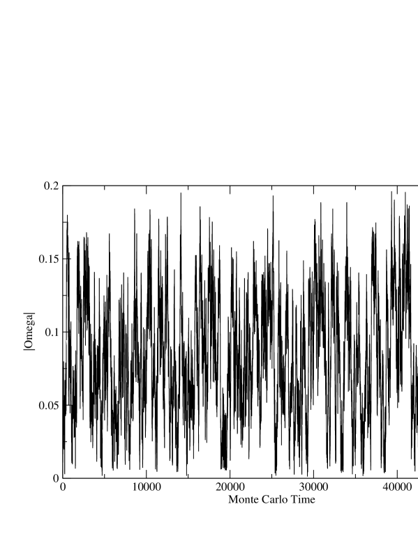
Figure 1: Evolution of $|\Omega|$ in Monte Carlo time. A unit in time is given by a cycle, consisting of one CM-Metropolis and 5 OV-Metropolis sweeps. We have simulated a $6\times 36^{3}$ lattice, at $\beta_{f}=7.803$, $\beta_{a}=-2.0$, with the modified weight that is specified in the text.

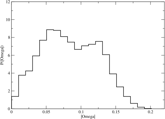
Figure 2: Histogram for the modified probability distribution for a $6\times 36^{3}$ lattice at $\beta_{f}=7.803$, $\beta_{a}=-2.0$. Details are given in the text.

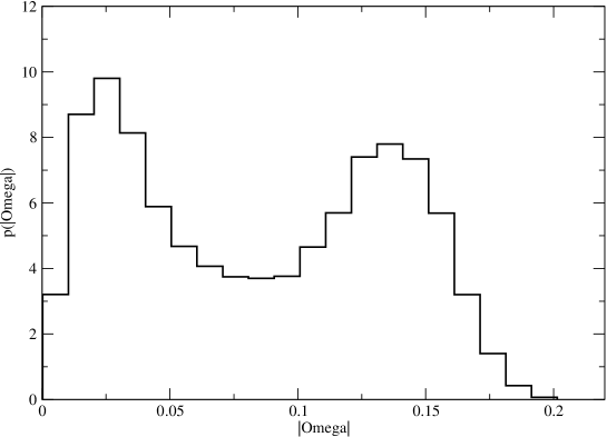
Figure 3: Histogram for the Boltzmann distribution $6\times 36^{3}$ lattice at $\beta_{f}=7.803$, $\beta_{a}=-2.0$. Details are given in the text.

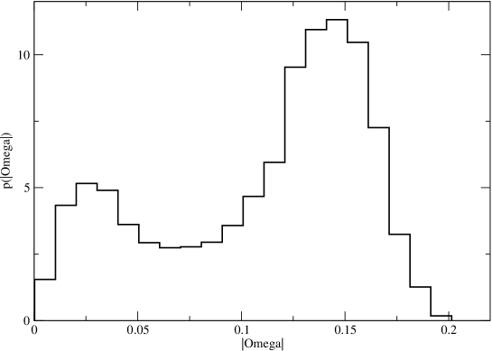
Figure 4: Histogram for the proper probability distribution $6\times 36^{3}$ lattice, simulated at $\beta_{f}=7.803$, $\beta_{a}=-2.0$, reweighted to $\beta_{f}=7.8056$. Details are given in the text.

Table 2: Summary of our results for the finite temperature phase transition obtained for the fundamental-adjoint gauge action. We give the value of $\beta_{f,c}$ for fixed values of $N_{t}$ and $\beta_{a}$. For a discussion of the numbers see the text.

$N_{t}$; $\beta_{a}$	00 0.0	–2.0	–4.0
2	5.0948(6)	6.4475(6)	7.8477(6)
3	5.5420(3)	7.1603(3)	8.8357(4)
4	5.6926(2)	7.4433(3)	9.2552(6)
6	000-	7.8056(5)	9.7748(11)

Table 3: Results for the finite temperature phase transition obtained by other authors for the standard Wilson gauge action, i.e. $\beta_{a}=0$.

$N_{t}$	$\beta_{f,c}$	ref.
2	5.0933(7)	[18]
3	–	–
4	5.6927(4)	[18]
4	5.69254(24)	[19]
4	5.6925(2)	[20]
6	5.89405(51)	[19]
6	5.8941(5)	[20]
8	6.0624(9)(3)	[20],[21]
12	6.3380(13)(10)	[20],[21]

Our results are summarized in Table 2. For comparison, we have collected results for $\beta_{a}=0$ from the literature. In contrast to our study, these results where obtained from the peak of the susceptibility. In the two cases, where we have mapping parameters, our results are consistent with those of the literature. For $\beta_{a}=0$, $N_{t}=6$ we performed no own simulation, but used in the following the result $\beta_{f}=5.89405(51)$ of ref. [19].

4.3 Lines of constant physics

At first order in perturbation theory the tree-level relation (8) is modified as [10]:

$$\beta_{W}=\beta_{f}+2\beta_{a}-5\frac{\beta_{a}}{\beta_{f}+2\beta_{a}}\;\;.$$ (26)

Up to higher order perturbative corrections and non-perturbative contributions, lines of constant $\beta_{W}$ should represent lines of constant physics.

Figure 5: Line of constant physics (solid line) as predicted by eq. (26) and the deconfinement transition line for $a=0.11\,\rm{fm}$ (open circles).

As a check of this relation, we compare in fig. 5 the values of the critical couplings for $N_{t}=6$, i.e. $a\simeq 0.11\,\rm{fm}$, with the one-loop prediction eq. (26), where we have set $\beta_{W}=\beta_{f,c}|_{a=0.11\,\rm{fm},\;\beta_{a}=0}$. For $\beta_{a}>0$ we adopt the results obtained in [5].
We see that the perturbative prediction fails in describing the line of constant physics. In ref. [5] it was observed that the prediction for positive $\beta_{a}$ can be considerably improved by using a tadpole improved perturbative formula. For negative $\beta_{a}$, however, the perturbative prediction seems to be completely unreliable. Hence we made no attempt to study tadpole improvement here.

Figure 6: Deconfinement transition lines for $a=0.11,0.17,0.33\,\rm{fm}$ and the interpolation formulas eq. (27) (solid lines). For $\beta_{a}>0$ the data are taken from ref. [5].

However, it turns out that the deconfinement transition lines can be parametrised quite well by a quadratic interpolation. Fitting the full range of available $\beta_{a}$ (including the results of ref. [5] for $\beta_{a}>0$) yields:

$$a=0.33\,\rm{fm}\,:\,\beta_{f} = 5.0948-0.6645\beta_{a}+0.0059\beta_{a}^{2}$$ (27)

$$a=0.17\,\rm{fm}\,:\,\beta_{f} = 5.6930-0.8586\beta_{a}+0.0080\beta_{a}^{2}$$

$$a=0.11\,\rm{fm}\,:\,\beta_{f} = 5.8951-0.9391\beta_{a}+0.0078\beta_{a}^{2}\;\;.$$

Fig. 6 shows the deconfinement transition lines for $a=0.11,0.17,0.33\,\rm{fm}$ for a range of positive and negative $\beta_{a}$. For $a=0.33\,\rm{fm}$, the interpolation formula reproduces the numerical values for $\beta_{a}<0$ within the statistical errors. For $a=0.17,0.11\,\rm{fm}$ and $\beta_{a}\leq 0$ the quadratic interpolation reproduced the numerical data only within two standard deviations.

5 The static potential

We have extracted the static potential from Polyakov loop correlation functions:

$$aV(r)=-\frac{1}{N_{t}}\left[\ln\langle P(x)^{*}P(y)\rangle+\epsilon\right]\;\;,$$ (28)

where $y=x+r\hat{1}$. $\epsilon$ is the correction due to excited states in the string spectrum. It vanishes exponentially as $N_{t}\rightarrow\infty$. In the free bosonic string approximation one gets [23, 24, 25, 26]

$$\epsilon=2\;\sum_{n=1}^{\infty}\ln(1-\exp[-\pi naN_{t}/r])\;\;.$$ (29)

Note that here, in contrast to the previous section, we are considering systems with a temporal extension $aN_{t}>>1/T_{c}$ to eliminate finite temperature corrections $\epsilon$ as much as possible. In the simulations reported below, we have chosen $N_{t}=6/(aT_{c})$. It is straightforward to check that for this choice, at our level of numerical precision, the corrections eq. (29) can be safely ignored.

We have computed the Polyakov loop correlation function with a variant of the algorithm that was recently proposed by Lüscher and Weisz [8]. Details of the algorithm are given below.

In this study, we consider rather coarse lattice spacings. Therefore the Sommer scale $r_{0}$ [22] is intrinsically affected by large systematic errors. On the other hand, we have computed the static potential up to rather large physical distances $r$. Therefore we decided to compute the string tension $a^{2}\sigma$ rather than $r_{0}/a$. We evaluated the string tension using the ansatz

$$V(r)=\sigma r+\mu-\frac{\pi}{12r}\left(1+\frac{b}{r}\right)$$ (30)

for the static quark potential, with $b=0.04{\rm fm}$ [8], where contributions of the order $O(r^{-3})$ are neglected. Details of our numerical analysis are given in the subsection 5.2.

5.1 Variant of the Lüscher and Weisz method to compute the Polyakov loop correlation function

In order to reach large values of $N_{t}$ we have implemented a variant of the recent proposal of Lüscher and Weisz [8]. In addition to the factorisation in temporal direction, we also use a factorisation in the spacial directions .

In temporal direction, we have used only one level of the factorisation. To this end, the lattice is divided in temporal direction into $N_{t}/N_{l}$ layers of the thickness $N_{l}$. Note that Lüscher and Weisz [8] also have used only one level of the factorisation in most of their numerical studies.

In addition, we have used a factorisation in the spacial directions. To this end, we have divided the lattice in blocks of the size $b^{3}\times N_{l}$. Within these blocks we consider only a subset of all possible Polyakov loops. See the two-dimensional sketch fig. 7 for an illustration. The idea of this choice is to use, for a given distance of the loops, only those loops that have a maximal distance from the boundaries of the blocks. In particular, for an even distance $r/a$ between the loops, we took the two loops with distance $(r/a)/2$ from the common boundary. For an odd distance $r/a$ between the loops, we took the distances $(r/a+1)/2$ and $(r/a-1)/2$ from the boundary between the blocks.

We have now a two-fold hierarchy of the algorithm. At the lowest level, we update at fixed boundaries of the blocks and fixed boundaries between the temporal slices. This step provides us with variance reduced segments of the Polyakov loops

$$\bar{P}(\vec{x},t_{0})=\frac{1}{M_{block}}\sum_{i=1}^{M_{block}}\prod_{t=t_{0}}^{t_{0}+N_{l}-1}U_{\vec{x},t,0}^{(i)}\;\;,$$ (31)

where $M_{block}$ is the number of updates that have been performed with fixed boundaries of the block and $i$ labels the configurations that have been generated this way. These variance reduced segments of the Polyakov loop could be viewed as a generalization of the multi-hit method for the variance reduction of a single link variable that has been applied in ref. [8].

Two of these variance reduced segments with the same $t_{0}$ from neighbouring spatial blocks are now used to construct the complex $9\times 9$ matrices of eq. (3.2) of ref. [8]:

$$\mathbb{T}(\vec{x},\vec{y},t_{0})_{\alpha,\beta,\gamma,\delta}=\bar{P}(\vec{x},t_{0})^{*}_{\alpha,\beta}\bar{P}(\vec{y},t_{0})_{\gamma,\delta}\;\;.$$ (32)

For fixed boundaries between the temporal layers, we perform a certain number of update sweeps before we repeat again the calculation of the variance reduced segments eq. (31). This procedure is performed $M_{layer}$ times and the matrix $\mathbb{T}$ is averaged over these $M_{layer}$ instances:

$$\bar{\mathbb{T}}(\vec{x},\vec{y},t_{0})_{\alpha,\beta,\gamma,\delta}=\frac{1}{M_{layer}}\sum_{j=1}^{M_{layer}}\mathbb{T}(\vec{x},\vec{y},t_{0})_{\alpha,\beta,\gamma,\delta}^{(j)}\;\;.$$ (33)

As in ref. [8], the Polyakov loop correlation function is now computed as

$$\langle P(x)^{*}P(y)\rangle\approx\frac{1}{M_{meas}}\sum_{k=1}^{M_{meas}}\left\{\prod_{t=0}^{t=N_{t}/N_{l}-1}\bar{\mathbb{T}}(\vec{x},\vec{y},tN_{l})^{(k)}\right\}_{\alpha,\alpha,\gamma,\gamma}\;\;,$$ (34)

where $M_{meas}$ is the number of complete measurement cycles. It is understood that measurements start after equilibration of the system.

In order to further improve the measurement of the segments of the Polyakov loop eq. (31) we have performed a multi-hit update of the single link variables. In addition, we have updated the links close to the centre of the block more frequently than those close to the boundary. To this end, we have set up a sequence of blocks inside the block having the sizes $(b-2)^{3}$, $(b-4)^{3}$, … . For each cycle (that consists of 2 OV-Metropolis and 2 CM-Metropolis sweeps over a block of the spatial size $(b-2m)^{3}$) we have performed $n$ such cycles for the next smaller block $(b-2(m-1))^{3}$. I.e. for each cycle of the full block ($b^{3}$), additional $n$, $n^{2}$, $n^{3}$… cycles are performed for the blocks of the spatial size $(b-2)^{3}$, $(b-4)^{3}$, $(b-6)^{3}$, … inside the block of the spatial size $b^{3}$. In most of our simulations we have chosen $n=3$. This way, of course, we can not gain exponentially, but we can fight, to some extend, the factor that we loose by the reduced number of Polyakov loops that we consider.

Compared with the original approach of Lüscher and Weisz, we gain the factorisation in the spacial directions. However, we lose a lot of copies of the correlator. Instead of $3\times N_{s}^{3}$ only $3\times(N_{s}/b)^{3}$ remain. To compensate partially for this fact, we update more frequently the links in the centre of the block than those at the boundary. A positive side-effect of the reduced number of copies of the Polyakov loop is that the memory requirements are drastically reduced compared with the original proposal.

Most of the CPU-time is spent with the block-boundaries fixed. This would allow for a rather trivial parallelisation on $(N_{t}/N_{l})(N_{s}/b)^{3}$ nodes. This makes the algorithm ideally suited for a PC-cluster equipped with a moderately fast interconnect like Gigabit-ethernet.

The obvious disadvantage of our variant of the algorithm is that even more parameters have to be tuned as in the original one of Lüscher and Weisz. In our case, it is almost unavoidable to make just ad hoc choices for some of the parameters. Finally, for the distances $r/a$ that we have reached, our method still seems to be slightly less efficient than the one of ref. [8]. Here is difficult to give a definite comparison, since we did not simulate at exactly the same parameters as ref. [8].

Figure 7: Two dimensional sketch of the block. Two of the spatial direction are show. The remaining spatial direction and the the temporal direction are perpendicular to the paper. Only the Polyakov loops that are indicated with black discs are computed.

Table 4: Parameters of our simulations to compute the static quark potential. In the first two columns we give the coupling constants. The third column contains the lattice sizes. In the fourth column the range of the distance $r$ is shown where the static potential has been computed. Finally we give the number of measurements $M_{meas}$, as defined in the previous section.

$\beta_{a}$	$\beta_{f}$	$N_{s}$, $N_{t}$	$r/a$	$M_{meas}$
0	5.0848	16, 12	2-6	30
–2	6.4475	16, 12	2-6	26
–4	7.8477	16, 12	2-6	24
0	5.5420	20, 18	2-8	17
–2	7.1603	20, 18	2-8	17
–4	8.8357	20, 18	2-8	21
0	5.6926	24, 24	2-10	56
–2	7.4433	18, 24	2-4	76
–4	9.2564	18, 24	2-4	1010
–4	9.254	18, 24	2-4	76

5.2 Numerical results for the string tension

To eliminate the constant $\mu$ in eq. (30) we consider the so called force

$$F(r)=\frac{\mbox{d}V}{\mbox{d}r}=\sigma+\frac{\pi}{12r^{2}}\left(1+\frac{2b}{r}\right)\;\;.$$ (35)

On the lattice, we compute the force from the potential either as

$$aF(r-a/2)=V(r)-V(r-a)$$ (36)

or

$$aF(r_{I})=V(r)-V(r-a)\;\;,$$ (37)

where $r_{I}$ is the tree-level improved distance defined in ref. [22].

In our numerical analysis, we made no attempt to compute $b$, but instead have used the result $b=0.04{\rm fm}$ of ref. [8]. In order to obtain the dimensionless quantity $a^{-1}b$ we have used $T_{c}r_{0}=0.7498(50)$ obtained in ref. [4] with $r_{0}=0.5{\rm fm}$. It follows

$$a(\{\beta_{f},\beta_{a}\}_{c})^{-1}b\approx 0.06N_{t}\;\;,$$ (38)

where here $a(\{\beta_{f},\beta_{a}\}_{c})N_{t}=1/T_{c}$. As a result, eq. (35) has no free parameters in addition to $\sigma$. Hence, for each value of $r/a$ we obtain an estimate for $a^{2}\sigma$.

We computed the static quark potential at the critical couplings that we have evaluated in the previous section for $\frac{1}{T_{c}a}=2,3,4$. The parameters of these simulations are given in Table 4. As thickness of the temporal layers we have used $N_{l}=1/(aT_{c})$ throughout. For the other parameters, let us just detail a typical example: For $\beta_{a}=0$, $\beta_{f}=5.6926$ we have used $M_{layer}=30$ and $M_{block}=40$.

In Table 5 we give details of our analysis of the force for $\beta_{a}=0$, $\beta_{f}=5.6926$, where we have collected our most accurate data. First we have estimated the string tension as $a(V(r)-V(r-a))$, ignoring the Lüscher term. We see that even for our largest values of $r/a$ the estimate does not stabilize. This behaviour is clearly improved, when the Lüscher term is used in the ansatz. Fortunately, the difference between the two definitions of the argument of the force eq.s (36,37) is only minor. Finally, we included $b=0.04{\rm fm}$ in the ansatz. As a result, the estimate of the string tension further stabilizes as the distance $r/a$ is varied. In fact, starting from $r/a=4$, all results are consistent within the statistical error.

As our final result we quote $a^{2}\sigma=0.162(1)$, which is obtained from the ansatz with $r_{I}$ and $b=0.04{\rm fm}$ at the distance $r/a=7$. Since the difference of our results with $b=0$ and $b=0.04{\rm fm}$ at $r/a=7$ is smaller than the statistical error, we are confident that the quoted error also covers possible systematic errors.

Table 5: Analysis of the force at $\beta_{a}=0$, $\beta_{f}=5.6926$. In this Table we give results obtained with various ansatze. In the second column we give the most naive estimate for the string tension $a^{2}\sigma$: $a(V(r)-V(r-a))$. In the third, we use the ansatz (35) in connection with eq. (36) and $b=0$. In the fourth column, the naive definition of the distance is replaced by the improved one eq. (37), still $b=0$. Finally, in the column 5 we use $b=0.04{\rm fm}$ as discussed in the text. In the last column we report the statistical error, which is the same in all cases.

$r/a$	$a^{2}\sigma_{naive}$	$a^{2}\sigma_{b=0}$	$a^{2}\sigma_{b=0}$,$r_{I}$	$a^{2}\sigma_{b=0.04{\rm fm}}$,$r_{I}$	stat. error
3	0.2211	0.1793	0.1707	0.1600	0.0003
4	0.1902	0.1688	0.1664	0.1629	0.0004
5	0.1783	0.1654	0.1645	0.1630	0.0004
6	0.1727	0.1640	0.1637	0.1629	0.0006
7	0.1692	0.1630	0.1628	0.1623	0.0006
8	0.1667	0.1621	0.1620	0.1617	0.0011
9	0.1655	0.1618	0.1618	0.1616	0.0025

We have extracted the final result for $a^{2}\sigma$ for the other values of the couplings in a similar fashion. In particular, we have always taken the result obtained with the tree-level improved distance $r_{I}$ and with $b=0.04{\rm fm}$. For $1/(aT_{c})=2$ and $3$, the final results for $a^{2}\sigma$ are taken from $r/a=4$ and $r/a=6$, respectively. In the case of $1/(aT_{c})=4$ we give the final result for $\beta_{a}=0$ and $\beta_{f}=5.6926$ that we obtained above. For $\beta_{a}=-2$ and $\beta_{a}=-4$ we do not have data for such large distances. Therefore we took $r/a=4$. The error that is quoted here includes a systematic error that we estimate based on our data for $\beta_{a}=0$ and $\beta_{f}=5.6926$. These results are summarized in Table 6.

M. Lüscher [28] has provided us with numerical data for the force at $\beta_{f}=5.7$, $\beta_{a}=0.0$ obtained on a $24\times 18^{3}$ lattice [8]. Using the procedure discussed above, we extract $a^{2}\sigma=0.156(1)$ from these data, where the error mainly covers possible systematic errors. (The statistical error of the force at $r/a=7$ is only $1.5\times 10^{-4}$). Extrapolating our data for $\beta_{f}=5.5420$, $\beta_{a}=0$ and $\beta_{f}=5.6926$, $\beta_{a}=0$, using the ansatz $\ln(a^{2}\sigma)=c+d\beta$, we get $a^{2}\sigma=0.1567(10)$ for $\beta_{f}=5.7$, $\beta_{a}=0$, which is consistent with the result that we have extracted from the numerical data of ref. [8, 28].

In Table 6 we also give the results for $T_{c}/\sqrt{\sigma}$, which are plotted in fig. 6 together with other values obtained for the Wilson action in [21]. The error of $T_{c}/\sqrt{\sigma}$ is dominated by the error of $a^{2}\sigma$.

Table 6: Summary of our final results for the string tension $a^{2}\sigma$ and the dimensionless ratio $T_{c}/\sqrt{\sigma}$. For a detailed discussion see the text.

$1/(aT_{c})$	$\beta_{a}$	$\beta_{f}$	$a^{2}\sigma$	$T_{c}/\sqrt{\sigma}$
2	0	5.0948	0.759(2)	0.574(1)
	–2	6.4475	0.742(2)	0.580(1)
	–4	7.8477	0.736(2)	0.583(1)
3	0	5.5420	0.319(2)	0.590(2)
	–2	7.1603	0.308(2)	0.601(2)
	–4	8.8357	0.306(2)	0.603(2)
4	0	5.6926	0.162(1)	0.621(2)
	–2	7.4433	0.160(1)	0.625(2)
	–4	9.2540	0.160(1)
	–4	9.2564	0.159(1)
	–4	9.2552		0.626(2)

We see that for $\beta_{a}=-2$ and $-4$ the estimate for $T_{c}/\sqrt{\sigma}$ is closer to the continuum limit than for $\beta_{a}=0$. However, the difference between $1/(aT_{c})=3$ and $1/(aT_{c})=4$ is larger than that for the different values of $\beta_{a}$ at fixed $1/(aT_{c})$. Since already for $1/(aT_{c})=4$ there is only a minor difference in the estimates for $T_{c}/\sqrt{\sigma}$ from $\beta_{a}=0$ and $\beta_{a}=-2$,$-4$, we decided to skip the determination of $a^{2}\sigma$ for $1/(aT_{c})=6$.

Figure 8: We have plotted our results for $T_{c}/\sqrt{\sigma}$ as a function of $1/N_{t}^{2}$, where $N_{t}=1/(aT_{c})$. In addition we give the results obtained in ref. [21] for $\beta_{a}=0$ at smaller lattice spacings.

For comparison, we have summarised in Table 7 continuum limit results for $T_{c}/\sqrt{\sigma}$ given in the literature that are obtained with various actions. In particular, the result of ref.s [21] and [31] are not compatible within the given error bars. Given that our smallest lattice spacing is $a\approx 0.17$ fm, we did not extrapolate our data to the continuum limit. However, looking at fig. 8, our data seem to be more compatible with a continuum result $T_{c}/\sqrt{\sigma}\approx 0.66$ than $0.63$.

Table 7: Results for the continuum limit of $T_{c}/\sqrt{\sigma}$ obtained with various lattice actions.

action	$T_{c}/\sqrt{\sigma}$
Wilson [21]	0.630(5)
Symanzik imp. [21]	0.634(8)
DBW2 [29]	0.627(12)
Iwasaki [30]	0.651(12)
1-loop tadpole impr. [31]	0.659(8)

6 Glueball masses

Table 8: Parameters of the glueball computation. For definitions see the text.

$\beta_{f}$	$\beta^{\prime}_{f}$	$\beta_{a}$	$N_{s}$	$N_{t}$	$n_{l}$	$N_{or}$	$N_{sub}$	$I_{sub}$	$I_{gl}$	$N_{meas}$
5.0948	-	–0.0	4	6	1,2,3,4	2	320	4	6	9931
6.4475	4.5	–2.0	4	6	1,2,3,4	2	160	2	6	19800
7.8477	4.5	–4.0	4	6	1,2,3,4	2	160	2	6	17800
5.5420	-	–0.0	6	8	2,4,6,8	4	160	4	8	4894
7.1603	5.0	–2.0	6	8	2,4,6,8	4	80	2	8	8500
8.8357	5.0	–4.0	6	8	2,4,6,8	4	80	2	8	7140
5.6926	-	–0.0	8	12	2,4,6,8	5	160	4	8	4520
7.4433	5.0	–2.0	8	12	2,4,6,8	5	80	2	8	2925
9.2564	5.0	–4.0	8	12	2,4,6,8	5	80	2	8	3852
05.89405	-	0	12	18	3,6,9,12	7	300	6	10	584
7.8056	5.0	-2.0	12	18	3,6,9,12	7	100	2	10	672
9.7748	5.0	-4.0	12	18	3,6,9,12	7	100	2	10	833

We continued our investigation of the lattice artefacts of the mixed action by measuring the mass (at zero temperature) of the lightest glueball $0^{++}$ at the critical values of $\beta_{f}$ for $\beta_{a}=0,-2,-4$ and $1/(aT_{c})=2,3,4,6$ that we have determined in section 4. This allows us to study the scaling of the dimensionless quantity $m_{0^{++}}/T_{c}$. The $0^{++}$ glueball mass is particularly interesting since it shows large lattice artefacts in the case of the Wilson action ($\beta_{a}=0$). The fact that the $0^{++}$ mass becomes very small at certain lattice spacings can be interpreted as the influence of the endpoint of the first order phase transition (see eq. (1)), where $m_{0^{++}}$ vanishes [6]. If this picture is correct, we expect that by choosing a negative $\beta_{a}$, we move away from the endpoint and hence the lattice artefacts on $m_{0^{++}}$ should be reduced.

In ref. [32] an action with 4 terms had been used: In addition to the plaquette in the fundamental representation, the plaquette in the adjoint representation, the representantion of dimension 6 and a $1times2$ loop in the fundamental representation were considered. All couplings except that of the fundamental plaquette were negative. The authors argue that this way the end-point of line of first order phase transtions in the fundamental-adjoint can be avoided. Their final estimate for the mass of the lightest glueball is $m_{0^{++}}/sqrt(\sigma)=3.5(3)$, which corresponds to $m_{0^{++}}r_{0}=4.07(35)$.

On anisotropic lattices ($a_{t}<<a_{s}$) the authors of ref. [33] found that by introducing in the action a term $\mbox{Re}\mbox{Tr}U_{P}(\vec{x},t,\mu,\nu)\;\mbox{Re}\mbox{Tr}U_{P}(vec{x},t+a_{t},\mu,\nu)$ for space-like plaquettes with a negative coupling constant, the scaling behaviour of the $0^{++}$ glueball mass can be improved. On top of this modification they [34] employed Symanzik-improvement [2, 3] with a $2\times 1$ Wilson loop term in the action.

In order to extract the mass $m_{0^{++}}$ of the $0^{++}$ glueball, we have computed the connected correlation function between spatial Wilson loops. To this end, we have chosen a basis of $N=7$ operators in the $A_{1}^{++}$ representation of the cubic group (among the 22 spatial Wilson loops up to lenght 8) plotted in fig. 9, which had shown the best signal-to-noise ratio in a previous study [4].

In order to get a better overlap with light states, we applied the APE smearing procedure to the spatial links [35]. For each operator, we used $M=4$ different smearing levels. For each shape with $d$ different orientations, we measured the observable

$$O_{l}(t)=\frac{N_{s}^{-3/2}}{\sqrt{d}}\sum_{\vec{x}}\sum_{n=1}^{d}{\rm Tr}W_{l}^{n}(\vec{x},t)\;\;,$$ (39)

where $W_{l}^{n}$ is the spatial Wilson loop with smearing level $l$, in the orientation $n$. We then constructed the correlation matrix

$$C_{ij}(t)=\langle O_{i}(t)O_{j}(0)\rangle-\langle O_{i}(t)\rangle\langle O_{j}(0)\rangle\;\;,$$ (40)

where now the indices $i,j$ run from 1 to $N\times M=28$.

Figure 9: Wilson loops used for the evaluation of $m_{0^{++}}$.

6.1 Factorization and error reduction

The exponential error reduction proposed by Lüscher and Weisz [8] and adopted in our work to compute Polyakov loop correlation functions, can be applied to a wider class of $n$-point functions. In particular, this idea has been tested on the Wilson loop correlation functions to compute the scalar and tensor glueball masses [9].

Here we have implemented only one level of factorisation. To this end, we divided the lattice in temporal direction into two sub-lattices with an extension $\Delta_{t}=N_{t}/2$ each. While keeping the spatial links at the time slices $t_{0}=1$ and $t_{1}=N_{t}/2+1$ fixed , we performed $\mathcal{N}_{sub}$ “sub-measurements”

$$\bar{O}_{i}(t)=\frac{1}{\mathcal{N}_{sub}}\sum_{n=1}^{\mathcal{N}_{sub}}{O}_{i}(t)^{(n)}\;\;.$$ (41)

For each of these measurements, we perform $I_{sub}$ sub-updating cycles. Every updating consists of one Cabibbo-Marinari heatbath sweep and $N_{or}$ overrelaxation sweeps. “Sub-updating” means that all link-variables except those at $t_{0}$ and $t_{1}$ are updated. The total number of sub-update cycles with one set of fixed link variables at $t_{0}$ and $t_{1}$ is then $N_{sub}=I_{sub}\mathcal{N}_{sub}$.

After these $N_{sub}$ sub-update cycles with fixed links at $t_{0}$ and $t_{1}$, we performed $I_{gl}$ global sweeps, with the same ratio $N_{or}$ between overrelaxation and heatbath sweeps. For $t$ even, we evaluated the 2-point “unsubtracted” correlation function as

$$C_{ij}^{u}(t)\approx\frac{1}{N_{meas}}\sum_{j=1}^{N_{meas}}\frac{1}{2}\sum_{t^{\prime}=1,N_{t}/2+1}\bar{O}_{i}(t^{\prime}+t/2)\;\bar{O}_{j}(t^{\prime}-t/2)$$ (42)

while for $t\geq 2$, $t$ odd, we used

$$C_{ij}^{u}(t)\approx\frac{1}{N_{meas}}\sum_{j=1}^{N_{meas}}\frac{1}{4}\sum_{t^{\prime}=1,N_{t}/2+1}\bar{O}_{i}(t^{\prime}+(t+1)/2)\;\bar{O}_{j}(t^{\prime}-(t-1)/2)\;\;\;$$

$$\;\;\;\;\;\;\;\;\;\;\;\;\;\;\;\;\;\;\;+\;\bar{O}_{i}(t^{\prime}+(t-1)/2)\;\bar{O}_{j}(t^{\prime}-(t+1)/2)\;\;,$$ (43)

where $N_{meas}$ is the number of times eq. (41) is evaluated. An important point on the subtraction of the vacuum expectation value is that only the measurements included in $C_{ij}^{u}(t)$ are taken into account. E.g. for $t$ even, we subtract

$$\frac{1}{N_{meas}^{2}}\left(\sum_{j=1}^{N_{meas}}\bar{O}_{i}(t^{\prime}+t/2)\right)\left(\sum_{j=1}^{N_{meas}}\bar{O}_{j}(t^{\prime}-t/2)\right)\;\;.$$ (44)

In this way, the two terms are highly statistically correlated, and hence statistical fluctuations cancel, when the difference is taken. For a more detailed discussion of this point see ref. [9]. Alternatively one could consider a temporal derivative of the correlation function, as proposed in ref. [45].

The free parameter of this 2-level scheme is the number of sub-measurements $\mathcal{N}_{sub}$. Here, we did not try to tune $\mathcal{N}_{sub}$ but rather followed the rule of ref. [9]:

$$\mathcal{N}_{sub}\simeq e^{m\overline{t}}\;\;,$$ (45)

where $m$ is the mass of the state that should be measured and $\overline{t}$ is the time, where we intend to extract the mass from the exponential decay of the 2-point function.

In fig. 10 we analyse the effective mass evaluated with the usual algorithm and with the factorisation formula for $\beta_{f}=5.6926$, $\beta_{a}=0$, up to $t=4$. For this purpose we collected 16000 measurements performed with the usual method and 400 measurements obtained with one level of factorisation, where each measurement is obtained with 40 sub-measurements. The computational effort for these two simulations is then roughly the same. The masses were extracted with the variational method discussed below. One can notice that for our choice of the algorithm, for $t=2$ the standard method is still more efficient that the variance reducing one. In our final analysis, we did not make use of the factorisation method for time separations $t=0,1$ and we computed the correlation function in the usual way. For $t\geq 3$ we observe however a substantial error reduction, and actually this is the region where we extract the glueball mass.

Figure 10: The plot shows the effective mass of the $0^{++}$ glueball at $\beta_{f}=5.6926$, $\beta_{a}=0$. In one case (squares) the correlation matrix has been calculated in the standard way, while in the other case (triangles) the variance reduction method that is discussed in the text has been applied. Note that for $t=1$ also the triangle result is computed in the standard way.

6.2 Analysis and results

As a first step, we symmetrised the correlation matrix by replacing $C_{ij}(t)$ by $1/2\left[C_{ij}(t)+C_{ji}(t)\right]$. The masses were extracted from the correlation functions by applying the usual variational method [37, 38]. We solved the generalised eigenvalue problem

$$C(t)\;v_{\alpha}(t,t_{0})=\lambda_{\alpha}(t,t_{0})\;C(t_{0})\;v_{\alpha}(t,t_{0})\;\;,$$ (46)

with $\alpha=0,...,(N\times M)-1$ and $\lambda_{0}>\lambda_{1}>...>\lambda_{(N\times M)-1}$. The indices $i,j$ of the correlation matrix $C(t)$ are now omitted. In our analysis, we have chosen $t_{0}=0$ throughout. We projected the correlation matrix on the ground state eigenvector computed for $t=t_{0}+1$

$$W(t)=v_{0}^{T}(t_{0}+1,t_{0})\;C(t)\;v_{0}(t_{0}+1,t_{0})\;,$$ (47)

and evaluated the effective mass using

$$m_{eff}(t)=\log\left(W(t-1)+\sqrt{W(t-1)^{2}-W(N_{t}/2)^{2}}\right)\;-$$ (48)

$$\log\left(W(t)+\sqrt{W(t)^{2}-W(N_{t}/2)^{2}}\right)\;,$$

which takes into account the periodic boundary conditions in temporal direction. In fig. 11 we show as an example the effective mass for $\beta_{f}=5.6926$, $\beta_{a}=0$ as a function of the distance $t$. We decided to extract the mass at $\overline{t}=4$, where the contributions of excited states should be smaller than the statistical errors. (Note that the mass of the first exited state in the $A_{1}^{++}$ channel is almost twice as heavy as the $0^{++}$ state.) Our final results are summarised in Table 9, together with the value of $\overline{t}$, where we extracted the masses.

Table 9: Results for the $0^{++}$ glueball mass in lattice units. As our final result, we have taken the effective mass evaluated at the distance $\overline{t}$.

$\beta_{f}$	$\beta_{a}$	$\overline{t}$	$am_{0^{++}}$	$m_{0^{++}}/T_{c}$
5.0948	–0.0	3	2.237(88)	4.47(18)
6.4475	–2.0	2	2.495(20)	4.990(40)
7.8477	–4.0	2	2.645(25)	5.290(50)
5.5420	–0.0	3	1.158(18)	3.474(54)
7.1603	–2.0	2	1.414(14)	4.242(42)
8.8357	–4.0	2	1.550(17)	4.650(51)
5.6926	–0.0	4	0.967(16)	3.868(64)
7.4433	–2.0	3	1.108(18)	4.432(72)
9.2564	–4.0	3	1.193(18)	4.772(72)
05.89405	4	–0.0	0.787(18)	4.72(11)
7.8056	–2.0	3	0.839(18)	5.03(11)
9.7748	–4.0	3	0.836(17)	5.02(10)

Figure 11: Effective mass for the $0^{++}$ state, at $\beta_{f}=5.6926$, $\beta_{a}=0$ as a function of the distance $t$.

Our final results for $m_{0^{++}}/T_{c}$ are also reported in Table 9. Here the dominant error is the uncertainty on $m_{0^{++}}$. Note that we computed the glueball mass for $\beta_{f}=9.2564,\beta_{a}=-4.0$, which was a preliminary estimate for the critical coupling $\beta_{f,c}$ and not the final result reported in Table 2. However, we estimate that the shift in the $0^{++}$ glueball mass corresponding to the shift in $\beta_{f}$ is negligible with respect to the statistical error. Fig. 12 shows $m_{0^{++}}/T_{c}$ as function of $(aT_{c})^{2}$.

For comparison, we give an estimate of the continuum limit based on the average of the following results given in the literature:

$m_{0^{++}}r_{0}$	ref.
4.35(11)	[40]
4.33(10)	[41]
4.21(11)(4)	[42]
4.23(22)	[43]
4.30(6)	average

The computation presented in [42] has been performed with anisotropic lattices. The results of [40] and [41] at a finite lattice spacing have been expressed in units of $r_{0}$ in ref. [48]. In ref. [40] further results are reported for which the continuum extrapolation has not been performed. Results for $m_{0^{++}}r_{0}$ at finite lattice spacing obtained with the FP (fixed point) action are also present [44]. The error that we give for the average should not taken too serious, since it is not clear, to which extend the error of the individual results is of systematic or statistic nature. In ref. [34] the authors plot their results for $m_{0^{++}}r_{0}$ obtained from anisotropic lattices with an improved action, as discussed above. They given no final result for the continuum limit. However, from the plot one reads off $m_{0^{++}}r_{0}\approx 4.0$ with a quite small error; incompatible with the average of the literature given above by several standard deviations.

Using the continuum limit relation [4]

$$T_{c}r_{0}=0.7498(50)$$ (49)

the average of the results from the literature can be converted to

$$m_{0^{++}}/T_{c}|_{a=0}=5.73(9)\;\;.$$ (50)

We made no attempt to extract a continuum result from our data, since it is quite clear from fig. 12 that corrections beyond $a^{2}$ are large. At $a\simeq 0.11{\rm fm}$ we do observe a moderate reduction of the lattice artefacts by using $\beta_{a}<0$ with respect to the usual Wilson action ($\beta_{a}=0$). For $\beta_{a}=0$, the deviation from the continuum result of eq. (50) amounts to $\sim 18\%$, while for $\beta_{a}=-2,-4$ it slightly decreases to $\sim 12\%$.
At $a\simeq 0.17{\rm fm}$ one observes discretization errors of $\sim 40\%$ for the Wilson action, while for the mixed action they amount to $\sim 25\%$ for $\beta_{a}=-2$ and $\sim 20\%$ for $\beta_{a}=-4$.

Figure 12: $m_{0^{++}}/T_{c}$ for $\beta_{a}=0$ (filled squares) $\beta_{a}=-2$ (open squares) and $\beta_{a}=-4$ (triangles) as function of $(aT_{c})^{2}$. The circle gives the continuum results extracted from the literature.

7 Summary and conclusions

We investigated the SU(3) lattice gauge model with a pure gauge action that contains plaquette terms in the fundamental and adjoint representation. In particular, we studied negative values of the adjoint coupling $\beta_{a}$. This choice is motivated by the presence of a first order phase transition line in the $(\beta_{f},\beta_{a})$ plane: one expects that moving towards negative $\beta_{a}$ the presence of the endpoint at $(\beta_{f},\beta_{a})=(4.00(7),2.06(8))$ becomes less important and hence that scaling and/or topological properties could be improved with respect to the Wilson action. These features would be highly desirable in view of upcoming simulations for fermionic actions with exact lattice chiral symmetry and in general for unquenched computations.

In section 4, we computed the critical coupling $\beta_{f,c}$ of the finite temperature deconfinement transition at $1/(aT_{c})=2,3,4,6$ and $\beta_{a}=0,-2,-4$ fixed. Since this measurement turned to be our most accurate, we have used $T_{c}$ to set the scale. We find that lines of constant physics, as predicted by one-loop perturbation theory, completely fail to describe our numerical results for negative $\beta_{a}$.

We then calculated the static quark potential from the Polyakov loop correlation funtion. To this end, we have implemented a variant of the algorithm recently proposed by Lüscher and Weisz. In addition to the factorisation in temporal direction, we have employed a factorisation in the spacial directions. This algorithm allowed us to compute the Polyakov loop correlation funtion up to $r\approx 1.5{\rm fm}$. Due to these large distances we were able to extract the string tension $\sigma$ with little systematic errors (section 5).

Studying the scaling behaviour of the quantity $T_{c}/\sqrt{\sigma}$ for the different $\beta_{a}$ at our disposal, we did not observe a significant improvement at negative adjoint couplings in comparison to the Wilson case $\beta_{a}=0$. The values obtained with negative $\beta_{a}$ are a little closer to the continuum limit.

In section 6 we computed the $0^{++}$ glueball mass for several lattice spacings and for $\beta_{a}=0,-2,-4$. Also for this computation we made use of the factorisation method to reduce the variance of the correlation function [9]. Although the efficiency here is not as spectacular as for the Polyakov loop correlation function, we were able to obtain a good statistical accuracy up to distances roughly twice the ones reached with the standard method.

It turns out that the mass $m_{0^{++}}$ of the lightest glueball is more sensitive to the variation of $\beta_{a}$. This had to be expected, since at the endpoint of the line of first order phase transitions the mass in lattice units is zero [6]. Therefore, in particular for $m_{0^{++}}$ large lattice artefacts should show up in the neighbourhood of the endpoint. We investigated the scaling behaviour of the dimensionless quantity $m_{0^{++}}/T_{c}$. Here indeed, we observed a significant reduction of the lattice artefacts for negative $\beta_{a}$. At $a\simeq 0.17\,{\rm fm}$, the lattice artefacts for $\beta_{a}=0$ are $~{}40\%$, while for $\beta_{a}=-4$ they decrease to $~{}20\%$.

In view of future dynamical QCD simulations, it would be interesting to study the effect on dislocations and to investigate spectrum of the Wilson-Dirac matrix obtained with the mixed action at negative $\beta_{a}$. Finally one should note that the hybrid-Monte-Carlo (HMC) algorithm can be easily implemented for the mixed fundamental-adjoint action.

8 Acknowledgements

M.H. thanks PPARC for support under the grant PPA/G/O/2002/00468. S.N. is supported by TMR, EC-Contract No. HPRNCT-2002-00311 (EURIDICE). Part of the study was conducted, while the authors have been members of the NIC and Theory group at DESY Zeuthen. We thank DESY and NIC/DESY for computational resources. We are grateful to R. Sommer for discussions in the initial phase of the project. We thank M. Lüscher for providing us unpublished data for the Polyakov loop correlation function. We are grateful to F. Gliozzi and O. Ogievetsky for advice on group-theory.

Appendix A Appendix: Is the transfer matrix positive?

In ref. [47] the transfer matrix for lattice QCD with the Wilson (fundamental) gauge action is constructed. It is straightforward to generalise this construction to the mixed fundamental/adjoint plaquette action.

In ref. [47] it is shown that the transfer matrix for the Wilson action is strictly positive if and only if

$$\int\mbox{d}U\int\mbox{d}U^{\prime}f^{*}(U)\;\exp\left(\frac{\beta_{f}}{2N}[\mbox{Tr}(U^{-1}U^{\prime})+\mbox{Tr}(U^{-1}U^{\prime})^{{\dagger}}]\right)f(U^{\prime})>0\;$$ (51)

for all square integrable, nonvanishing functions $f$ on the gauge group SU(3).

This can be generalized as

$$\int\mbox{d}U\int\mbox{d}U^{\prime}f^{*}(U)\;\exp\left(\frac{\beta_{f}}{2N}[\mbox{Tr}V+\mbox{Tr}V^{{\dagger}}]+\frac{\beta_{a}}{N^{2}}\mbox{Tr}V\;\mbox{Tr}V^{{\dagger}}\right)\;f(U^{\prime})>0$$ (52)

where $V=U^{-1}U^{\prime}$.

Following ref. [47], the integration kernel of eq. (52) can be expanded in a Fourier series on the group

$$\exp\left(\frac{\beta_{f}}{2N}[\mbox{Tr}V+\mbox{Tr}V^{{\dagger}}]+\frac{\beta_{a}}{N^{2}}\mbox{Tr}V\;\mbox{Tr}V^{{\dagger}}\right)\;=\;\sum_{\nu}c_{\nu}\chi^{(\nu)}(V)\;,$$ (53)

where the sum runs over the set of all irreducible representations of SU(3) and $\chi^{(\nu)}(V)$ is the character of the representation $\nu$. In order that eq. (52) holds, it is necessary and sufficient that all coefficients $c_{\nu}>0$ are positive. For $\beta_{f}>0$ and $\beta_{a}=0$ it is proven [47] that this is indeed the case:

$$\exp\left(\frac{\beta_{f}}{2N}[\mbox{Tr}V+\mbox{Tr}V^{{\dagger}}]\right)\;=\;\sum_{n,m=0}^{\infty}a_{nm}(\mbox{Tr}V)^{n}(\mbox{Tr}V^{\dagger})^{m}\;\;,$$ (54)

where $a_{nm}>0$. Here, $(\mbox{Tr}V)^{n}(\mbox{Tr}V^{\dagger})^{m}$ is the trace of the tensor product representation of SU(3) composed of $n$ quark and $m$ antiquark representations. Reducing out the tensor product, one gets

$$(\mbox{Tr}V)^{n}(\mbox{Tr}V^{\dagger})^{m}\;=\;\sum_{\nu}c_{\nu}(n,m)\chi^{(\nu)}(V)\;\;,$$ (55)

where $c_{\nu}(n,m)>0$. Since all irreducible representations can be obtained by reducing out tensor products of quark representations, $c_{\nu}>0$ for all $\nu$. It is trivial to extend this prove to $\beta_{f}>0$ and $\beta_{a}\geq 0$.

However for $\beta_{a}<0$, as we consider here, the situation becomes more complicated. In the expansion

$$\exp\left(\frac{\beta_{f}}{2N}[\mbox{Tr}V+\mbox{Tr}V^{{\dagger}}]+\frac{\beta_{a}}{N^{2}}\mbox{Tr}V\;\mbox{Tr}V^{{\dagger}}\right)\;=\sum_{n,m=0}^{\infty}a_{nm}(\mbox{Tr}V)^{n}(\mbox{Tr}V^{{\dagger}})^{m}$$ (56)

it is no longer guaranteed that $a_{nm}>0$ for all choices of $n,m$. This can be most easily seen for

$$a_{n,1}=\frac{1}{(n+1)!}(n+1)\left[\frac{\beta_{f}}{2N}\right]^{n+1}+\frac{1}{n!}n\left[\frac{\beta_{f}}{2N}\right]^{n-1}\frac{\beta_{a}}{N^{2}}\;\;.$$ (57)

It follows that $a_{n,1}$ is positive for $(\beta_{f}/2)^{2}/n+\beta_{a}>0$. I.e. as $n$ increases, the lower limit on $\beta_{a}$ goes to zero. However, it remains quite unclear how the $a_{n,m}$ will add up in the coefficients $c_{\nu}$ and whether $c_{\nu}>0$. We were not able to clarify this question rigorously.

To get some idea, we evaluated the coefficients $c_{\nu}$ for the pairs of $\beta_{f},\beta_{a}$ studied in this paper, for representations $\nu$ up to the dimension 15.

To this end we evaluated the integrals

$$c_{\nu}=\int\mbox{d}V\chi_{\nu}^{*}(V)\exp\left(\frac{\beta_{f}}{2N}[\mbox{Tr}V+\mbox{Tr}V^{{\dagger}}]+\frac{\beta_{a}}{N^{2}}\mbox{Tr}V\;\mbox{Tr}V^{{\dagger}}\right)\;$$ (58)

numerically. It turned out that $c_{\nu}>0$ for all coefficients that we computed, except for the coefficient of one 15 dimensional representation at $\beta_{f}=7.8477$ and $\beta_{a}=-4$.

We applied a second numerical approach to check the positivity of the integration kernel. Assume that we perform the integration eq. (52) with a Monte Carlo method. I.e. we evaluate $f(U)$ for $m$ SU(3) matrices that have been selected randomly. Choosing the same SU(3) matrices for both integrations, the integration kernel becomes a real symmetric $m\times m$ matrix. In this study, we have used $m\leq 10000$.

To check the positivity of this matrix, we evaluated its smallest eigenvalue. It turned out that for $\beta_{a}=-2$ and $\beta_{a}=-4$ and all values of $\beta_{f}$ that we have studied here, negative eigenvalues are found. However, in particular for $\beta_{a}=-2$, the absolute value of the smallest eigenvalue is by several orders of magnitude smaller than the largest eigenvalue. Notice that no quantitative sign of a violation of positivity has been observed in the decay of the Wilson loop correlation functions, while for the improved actions studied in ref. [4] such violations were clearly visible. It remains an open question, whether there is a finite range of negative $\beta_{a}$, where the transfermatrix is strictly positive.

References

- [1] Ch. Gattringer et al. (BGR Collaboration), Nucl.Phys. B 677 (2004) 3, hep-lat/0307013.
- [2] K. Symanzik, Nucl.Phys. B 226 (1983) 187 205.
- [3] M. Lüscher and P. Weisz, Phys.Lett. B 158 (1985) 250.
- [4] Silvia Necco, Nucl.Phys. B 683 (2004) 137, hep-lat/0309017.
- [5] T. Blum, C. DeTar, U. M. Heller, L. Kärkkäinen, K. Rummukainen and D. Toussaint, Nucl.Phys. B 442 (1995) 301, hep-lat/9412038.
- [6] U. M. Heller, Phys.Lett. B 362 (1995) 123, hep-lat/9508009; Nucl.Phys.Proc.Suppl. 47 (1996) 262, hep-lat/9509010.
- [7] Y. Iwasaki, Nucl.Phys. B 258 (1985) 141; Univ. of Tsukuba report, UTHEP-118 (1983), unpublished.
- [8] M. Lüscher and P. Weisz, JHEP 0109 (2001) 010, hep-lat/0108014; JHEP 0207 (2002) 049, hep-lat/0207003.
- [9] H. B. Meyer, JHEP 301 (2003) 48, hep-lat/0209145; JHEP 0401 (2004) 030, hep-lat/0312034.
- [10] A. Gonzales-Arroyo and C.P. Korthals Altes, Nucl.Phys. B 205 [FS5] (1982) 46.
- [11] N. Cabibbo and E. Marinari, Phys.Lett. B 119 ( 1982) 387.
- [12] R. Petronzio and E. Vicari, Phys.Lett. B 245 (1990) 581.
- [13] M. Lüscher, Comput.Phys.Commun. (1994) 100, hep-lat/9309020.
- [14] A.M. Polyakov, Phys.Lett. B 72 (1978) 477.
- [15] L. Susskind, Phys.Rev. D 20 (1979) 2610.
- [16] C. Borgs, Int.J.Mod.Phys. C 3 (1992) 897 and refs. therein.
- [17] B. Berg and T. Neuhaus, Phys.Lett. B 267 (1991) 249; hep-lat/9202004, Phys.Rev.Lett. 68 (1992) 9.
- [18] N. A. Alves, B. A. Berg and S. Sanielevici, Nucl.Phys. B 376 (1992) 218.
- [19] Y. Iwasaki, K. Kanaya, T. Yoshié, T. Hoshino, T. Shirakawa, Y. Oyanagi, S. Ichii and T. Kawai, Phys.Rev. D 46 (1992) 4657.
- [20] G. Boyd, J. Engels, F. Karsch, E. Laermann, C. Legeland, M. Lutgemeier and B. Petersson, Nucl.Phys. B (1996) 469, hep-lat/9602007.
- [21] B. Beinlich, F. Karsch, E. Laermann and A. Peikert, Eur.Phys.J. C 6 (1999) 133, hep-lat/9707023.
- [22] R. Sommer, Nucl.Phys. B 411 (1994) 839, hep-lat/9310022.
- [23] M. Minami, Prog.Theor.Phys. 59 (1978) 1709.
- [24] K. Dietz and T. Filk, Phys.Rev. D 27 (1983) 2944.
- [25] M. Flensburg and C. Peterson, Nucl.Phys. B 283 (1987) 141.
- [26] P. de Forcrand, G. Schierholz, H. Schneider and M. Teper, Phys.Lett. B 160 (1985) 137.
- [27] M. Laine, H.B. Meyer, K. Rummukainen and M. Shaposhnikov, JHEP 0404 (2004) 027, hep-ph/0404058.
- [28] M. Lüscher, private communication.
- [29] QCD-TARO collaboration, Ph. de Forcrand et al. , Nucl.Phys. B 577 (2000) 263, hep-lat/9911033.
- [30] CP-PACS, M. Okamoto et al., Phys.Rev. D 60 (1999) 094510, hep-lat/9905005.
- [31] D. W. Bliss, K. Hornbostel, and G. P. Lepage, hep-lat/9605041.
- [32] R. Gupta, A. Patel, C. F. Baillie, G. W. Kilcup and S. R. Sharpe, Phys.Rev. D 43 (1991) 2301 and refs. therein.
- [33] C. Morningstar and M. Peardon, Nucl.Phys. B (Proc.Suppl.) 73 (1999) 927, hep-lat/9808045.
- [34] C. Morningstar and M. Peardon, Nucl.Phys. (Proc.Suppl.) 83 (2000) 887, hep-lat/9911003 and nucl-th/0309068.
- [35] APE collaboration, M. Albanese et al., Phys.Lett. B 192 (1987) 163.
- [36] C. Michael and J. Peisa, Phys.Rev. D 58 (1998) 034506, hep-lat/9802015.
- [37] N. A. Campbell, C. Michael and P. E. L. Rakow, Phys.Lett. B 139 (1984) 288.
- [38] M. Lüscher and U. Wolff, Nucl.Phys. B 339 (1990) 222.
- [39] P. Majumdar, Nucl.Phys. B664 (2003) 213, hep-lat/0211038.
- [40] M. J. Teper, Glueball masses and other physical properties of SU(N) gauge theories in D = (3+1): A Review of lattice results for theorists, hep-th/9812187.
- [41] A. Vaccarino and D. Weingarten,Phys. Rev. D 60 (1999) 114501, hep-lat/9910007.
- [42] C. J. Morningstar and M. J. Peardon, Phys.Rev. D 60, hep-lat/9901004.
- [43] C. Liu, Commun.Theor.Phys. 35 (2001) 288.
- [44] F. Niedermayer, P. Rufenacht and U. Wenger, Nucl.Phys. B 597 (2001) 413, hep-lat/0007007.
- [45] P. Majumdar, Y. Koma and M. Koma, Nucl.Phys. B 677 (2004) 273, hep-lat/0309003.
- [46] ALPHA collaboration (Marco Guagnelli et al.). Nucl.Phys.B 535 (1998) 389, hep-lat/9806005.
- [47] M. Lüscher, Commun.Math.Phys. 54 (1977) 283.
- [48] H. Wittig, Lattice gauge theory, hep-ph/9911400.