Hadronic property at finite density

Abstract

We report on three topics on finite density simulations: (i) the derivative method for hadronic quantities, (ii) phase fluctuations in the vicinity of the critical temperature and (iii) the density of states method at finite isospin density.

1 Introduction

Lattice QCD simulations at finite chemical potential $\mu$ are extremely difficult due to the sign problem. Recently it has been realized that at small chemical potential one can study density effects on physical quantities by various approaches[1]. One of the approaches is the derivative method which has been used for the study of response of meson masses with respect to $\mu$ by QCD-TARO collaboration[2, 3]. The original idea of the derivative method may date back to the study of the fermion number susceptibilities[4] where the derivative of the fermion number density with repect to $\mu$ were calculated. In section 2, we report on results from the derivative method for the response of meson masses as well as the chiral condensate.

At large $\mu$ we believe that the standard Monte Calro method based on importance sampling fails due to the sign problem, i.e. the phase fluctuation is expected to be large for large $\mu$. However, we do not know exactly how the phase fluctuates with various simulation parameters. In section 3, we give results of the phase fluctuation in the vicinity of the critical temperature. We also present results of $\langle\bar{\psi}\psi\rangle$ and the Polyakov loop for $\mu\leq 0.25$.

The most lattice simulations have been performed by methods based on importance sampling. There exists an alternative method called density of states method. An advantage of the density of states method is that one can obtain results for various values of simulation parameters without making independent simulations although the lattice size may be limited to a small one. In section 4, we give results from the density of states method for isospin density. Since the system at isospin density has no sign problem the results are compared with those from the standard Monte Carlo method.

2 Derivative method for hadronic quantities

The derivative method extracts physical information at a small chemical potential without directly simulating a system at finite chemical potential. The original idea of the derivative method comes from the calculations of the fermion number susceptibilities[4]. The QCD-TARO collaboration[2, 3] studied the response of meson masses by the derivative method. The method was also used for the study of the pressure[5, 6].

Let us consider an observable $O(\mu)$. The expectation value of the observable $O(\mu)$ is given by

$$<O>=\frac{\int O\Delta e^{-S_{g}}dU}{\int\Delta e^{-S_{g}}dU},$$ (1)

where $S_{g}$ is the gluonic action and $\Delta$ stands for the fermion determinant. For two flavors of staggered quarks (u and d quarks), $\Delta$ is written as

$$\Delta = \det M(\mu_{u})^{1/4}\det M(\mu_{d})^{1/4}$$ (2)

$$= \exp(\frac{1}{4}TrlnM(\mu_{u})+\frac{1}{4}TrlnM(\mu_{d})).$$ (3)

The first derivative of $\langle O\rangle$ with respect to $\mu$ at $\mu=0$ is given by

$$\frac{\partial\langle O\rangle}{\partial\hat{\mu}}=\langle\dot{O}+O\frac{\dot{\Delta}}{\Delta}\rangle,$$ (4)

where we used $\displaystyle\dot{O}=\frac{\partial O}{\partial\mu}$ for simplicity. Note that here we used $\displaystyle\langle\frac{\dot{\Delta}}{\Delta}\rangle=0$ at $\mu=0$. Similarly the second derivative at $\mu=0$ is given by

$$\frac{\partial^{2}<O>}{\partial\mu^{2}}=<\ddot{O}+2\dot{O}\frac{\dot{\Delta}}{\Delta}>-<O\circ\frac{\ddot{\Delta}}{\Delta}>_{cc},$$ (5)

where $<A\circ B>_{cc}=<AB>-<A><B>$.

Next let us consider the spatial hadronic correlator,

$$C(x)\equiv\sum_{y,z,t}\langle H(x,y,z,t)H(0,0,0,0)^{\dagger}\rangle,$$ (6)

and take derivatives of $C(x)$. We assume that $C(x)$ is dominated by a single pole contribution,

$$C(x)=A(e^{-Mx}+e^{-M(L-x)}),$$ (7)

where $M$ is the hadron mass and $L$ is the lattice size in the $x$ direction. Taking the first and the second derivatives of $C(x)$ with respect to $\mu$ we obtain

$$\frac{1}{C(x)}\frac{dC(x)}{d\mu}=\frac{1}{A}\frac{dA}{d\mu}+\frac{dM}{d\mu}\times\{(x-\frac{L}{2})\tanh[M(x-\frac{L}{2})]-\frac{L}{2}\},$$ (8)

and

$$\frac{1}{C(x)}\frac{d^{2}C(x)}{d\mu^{2}} = \frac{1}{A}\frac{d^{2}A}{d\mu^{2}}+(\frac{2}{A}\frac{dA}{d\mu}\frac{dM}{d\mu}+\frac{d^{2}M}{d\mu^{2}})\{(x-\frac{L}{2})\tanh[M(x-\frac{L}{2})]-\frac{L}{2}\}$$

$$+ (\frac{dM}{d\mu})^{2}\{(x-\frac{L}{2})^{2}+\frac{L^{2}}{4}-L(x-\frac{L}{2})\tanh[M(x-\frac{L}{2})]\}.$$

The left hand sides of these equations are used as fitting functions to the Monte Carlo data given by eq.(4) and (5). The response of masses with respect to $\mu$, i.e. $\displaystyle\frac{dM}{d\mu}$ and $\displaystyle\frac{d^{2}M}{d\mu^{2}}$ are given as the fitting parameters.

The QCD-TARO collaboration studied the response of the pseudo scalar (PS) meson screening mass for $n_{f}=2$ flavors on $16\times 8^{2}\times 4$ lattices. The first response of the PS meson mass turned out to be consistent with zero. Thus the first relevant response is the second one. Figure 1 shows the second responses of the PS meson mass.

Figure 1: Second responses $d^{2}M/d\mu_{S}^{2}$ and $d^{2}M/d\mu_{V}^{2}$ of the PS meson mass at $m_{q}a=0.025$ as a function of $T/T_{c}$[2, 3].

Here the isoscalar and isovector chemical potentials are defined by

$$\mu_{S}=\mu_{u}=\mu_{d},$$ (10)

and

$$\mu_{V}=\mu_{u}=-\mu_{d},$$ (11)

respectively. The isovector chemical potential is also called isospin chemical potential and we also use $\mu_{V}$ to stand for the isospin chemical potential.

In the low temperature phase, the dependence of the mass on $\mu_{S}$ is small. This behavior is to be expected since below $T_{c}$ the PS meson is a Goldstone boson and persists its zero mass feature. On the other hand, above $T_{c}$ the PS meson loses the Goldstone nature and can obtain its mass, as a result $d^{2}M/d\mu_{S}^{2}$ seems to remain finite.

The PS meson on $\mu_{V}$ seems to behave differently. In the low temperature phase the PS meson mass tends to decrease with $\mu_{V}$. In the high temperature phase the PS meson also seems to decrease but the rate of the decrease is small.

Next we consider the derivatives of $\langle\bar{\psi}\psi\rangle$. At $\mu=0$ the first derivatives of $\langle\bar{\psi}\psi\rangle$ with respect to both isoscalar and isovector chemical potentials are identically zero, i.e.

$$\frac{\partial\langle\bar{\psi}\psi\rangle}{\partial\mu_{S}}=\frac{\partial\langle\bar{\psi}\psi\rangle}{\partial\mu_{V}}=0.$$ (12)

     

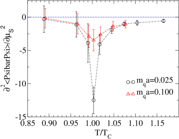
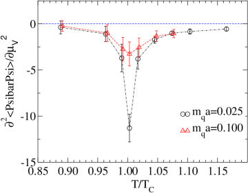
Figure 2: $\displaystyle\frac{\partial^{2}\langle\bar{\psi}\psi\rangle}{\partial\mu_{S}^{2}}$ (left) and $\displaystyle\frac{\partial^{2}\langle\bar{\psi}\psi\rangle}{\partial\mu_{V}^{2}}$ (right) as a function of $T/T_{c}$[7].

Thus the first relevant term is the second derivative. Figure 2 shows the second derivatives of $\langle\bar{\psi}\psi\rangle$ with respect to $\mu_{S}$ and $\mu_{V}$ for $n_{f}=2$ flavors on $16\times 8^{2}\times 4$ lattices, calculated by Choe et al.[2, 7]. No significant difference can be seen between $\displaystyle\frac{\partial^{2}\langle\bar{\psi}\psi\rangle}{\partial\mu_{S}^{2}}$ and $\displaystyle\frac{\partial^{2}\langle\bar{\psi}\psi\rangle}{\partial\mu_{V}^{2}}$. The strength of the responses increases as the quark mass decreases. The similar results are also obtained for the NJL model[8].

The results of the second derivatives can be used for evaluating $\langle\bar{\psi}\psi\rangle$ at small chemical potentials as

$$\langle\bar{\psi}\psi(\mu)\rangle\approx\langle\bar{\psi}\psi(0)\rangle+\frac{1}{2}\frac{\partial^{2}\langle\bar{\psi}\psi\rangle}{\partial\mu^{2}}\mu^{2}.$$ (13)

Figure 3: $\langle\bar{\psi}\psi\rangle$ extrapolated to finite $\mu_{S}$ at $m_{q}=0.025$[7]. Here $T_{c}$ is the critical temperature at $\mu=0$.

Figure 3 shows $\langle\bar{\psi}\psi(\mu_{S})\rangle$ extrapolated to finite $\mu_{S}$ using eq.(13). We see that qualitatively the critical temperature decreases as $\mu$ increases. Similar behavior can be seen for the case of the isovector chemical potential.

3 Phase fluctuation in the vicinity of the critical temperature

There is no satisfactory method to simulate the system at large $\mu$. In principle the reweighting method can be applied for any $\mu$ as

$$\langle O(\mu)\rangle=\frac{\langle O(\mu)e^{i\theta}\rangle_{\mu_{V}}}{\langle e^{i\theta}\rangle_{\mu_{V}}},$$ (14)

where $\displaystyle\langle O\rangle_{\mu_{V}}$ stands for the expectation value of the operator $O$ in an ensemble at isospin density, i.e. the configurations are generated with the phase quenching measure $\sim|\det M(\mu)|^{n_{f}/4}e^{-S_{g}}$. For large $\mu$ eq.(14) is expected to be impractical since $\langle e^{i\theta}\rangle_{\mu_{V}}$ becomes small. For such small $\langle e^{i\theta}\rangle_{\mu_{V}}$, in order to obtain a meaningful value of eq.(14) one needs extremely high statistics. Furthermore there is another difficulty: the calculation of the complex phase $\theta$ contains a determinant calculation which is computationally costly. For small $\mu$ one may use the Taylor expansion of the determinant as[9]

$$\det M(\mu)=\exp(TrlnM(0)+\left.Tr\frac{1}{M}\frac{\partial M}{\partial\mu}\right|_{\mu=0}\times\mu+O(\mu^{2})).$$ (15)

The first term of eq.(15) is real and the second term is pure imaginary. Thus $\theta$ at small $\mu$ is given by

$$\theta=\bar{\theta}+O(\mu^{3}),$$ (16)

where

$$\bar{\theta}=\left.ImTr\frac{1}{M}\frac{\partial M}{\partial\mu}\right|_{\mu=0}\times\mu.$$ (17)

In this expression no determinant calculation is required. Instead, $\bar{\theta}$ is given by a trace calculation and the computational cost is much reduced. An empirical study shows that the quality of the approximation $\bar{\theta}$ is valid for $\mu\leq 0.2$[10]. Figure 4 shows $\bar{\theta}$ vs the exact phase $\theta$.

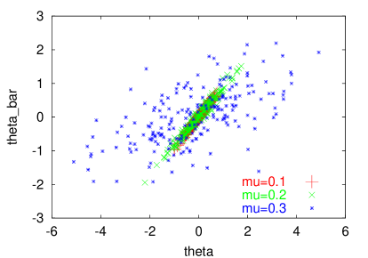
Figure 4: $\bar{\theta}$ vs the exact phase $\theta$ for 3 values of $\mu$[10].

The agreement between $\bar{\theta}$ and $\theta$ is excellent for $\mu=0.1$ and 0.2. However for $\mu=0.3$, $\bar{\theta}$ deviates from the exact value $\theta$.

For large $\mu$, in order to obtain $\theta$, using the approximation is not sufficient and one needs the determinant calculation to obtain the value of $\theta$. Sasai, Nakamura and Takaishi studied the phase fluctuations by calculating $\theta$ without any approximation. Figure 5 shows the phase fluctuation $\langle\cos(\theta/2)\rangle_{\mu_{V}}$ for $n_{f}=2$ as a function of $\beta$[11]. $\langle\cos(\theta/2)\rangle_{\mu_{V}}$ is the average value over the phase quenched ensemble. The phase fluctuation increases, i.e., $\langle\cos(\theta/2)\rangle_{\mu_{V}}$ decreases as $\mu$ increases. However in the deconfinement region, the phase fluctuation is much smaller than that in the confinement region.

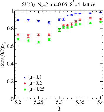
Figure 5: Phase fluctuation $\langle\cos(\theta/2)\rangle_{\mu_{V}}$ for $n_{f}=2$ in the isospin ensemble[11]. $\beta_{c}(\mu=0)\approx 5.32$.

With the simulation parameters used here, the phase fluctuation is not significantly large and the expectation values at finite $\mu$ can be obtained by the reweighting from the isospin ensemble as eq.(14). Figure 6 shows $\langle\bar{\psi}\psi\rangle$ and Polyakov loop with and without reweighting for $\mu\leq 0.25$. We do not see any difference between the results with and without reweighting. This is consistent with the result of $\langle\bar{\psi}\psi\rangle$ in Toussaint. This might indicate that for $\mu\leq 0.25$ the phase effects are small. This fact is also consistent with that the phase diagram obtained at small $\mu_{V}$ is similar to that at small $\mu_{S}$[14, 13]. The phase diagram at small $\mu_{V}$ was calculated for $n_{f}=2$ staggered fermions[14] and also for the Wilson fermions[13] with the plaquette and DBW2[15, 16, 17] gauge actions.

   

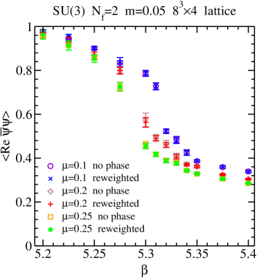
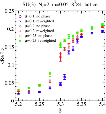
Figure 6: $\langle\bar{\psi}\psi\rangle$ (left) and Polyakov loop (right) with and without reweighting[11].”no phase” stands for the results without reweighting.

Although the isospin system has a positive measure and can be simulated with the standard Monte Carlo methods, for large chemical potentials we face the computational difficulty: the matrix solver does not converge. As a result the simulation can not be performed. This feature is also mentioned in Toussaint. Interestingly for further large chemical potentials $\mu>\mu_{c}$ ($\mu_{c}$ is a certain value which is dependent of the simulation parameters), the matrix solver converges[18].

4 Density of states method at isospin density

The most lattice simulations are performed by the Monte Carlo methods based on importance sampling. Here we report on an alternative approach, the density of states (DOS) method. We apply the DOS method for isospin density and compare the results with those from the standard Monte Carlo method.

The DOS method has been applied for gauge theories[19] and QED with dynamical fermions[20]. Luo[21] applied the DOS method for QCD and argued that if the eigenvalues of the Dirac operators are determined the thermodynamic quantities derived from the partition function can be evaluated at any quark mass and flavor.

The expectation value of the operator $O$ is given by

$$\langle O\rangle=\frac{1}{Z}\int[dU]O[U]\det M(m_{q},\mu)^{n_{f}/4}\exp(-\beta S_{g}[U]),$$ (18)

where $M(m_{q},\mu)$ is assumed to be a staggered fermion matrix at quark mass $m_{q}$ and at chemical potential $\mu$. We define $n(E)$ as

$$n(E)=\int[dU]\delta(6VE-S_{g}[U]),$$ (19)

where $V$ is the number of lattice sites and $E$ is the plaquette energy.

Using $n(E)$, $\langle O\rangle$ is expressed by

$$\langle O\rangle=\frac{1}{Z_{n}}\int dEn(E)e^{-\beta 6VE}\langle O\det M(\mu)^{N_{f}/4}\rangle_{E},$$ (20)

where

$$Z_{n}=\int dEn(E)e^{-\beta 6VE}\langle\det M(\mu)^{N_{f}/4}\rangle_{E}.$$ (21)

$\langle\bullet\rangle_{E}$ stands for the microcanonical averages with fixed $E$. If these microcanonical averages are determined as a function of $E$, $\langle O\rangle$ is given at any $\beta$. Furthermore, Luo argued that if one stores the eigenvalues of $M(\mu)$ for all configurations, then one can evaluate $\langle\det M(\mu)^{N_{f}/4}\rangle_{E}$ at any quark mass and flavor as

$$\langle\det M(\mu)^{N_{f}/4}\rangle_{E}=\langle(\prod_{i}^{N_{c}V}(\lambda_{i}(\mu)+m_{q}))^{N_{f}/4}\rangle_{E},$$ (22)

where $\lambda_{i}(\mu)$ is the i-th eigenvalue of the massless fermion matrix $M(m_{q}=0)$ and $N_{c}=3$ for SU(3). On the other hand, in general $\langle O\det M(\mu)^{N_{f}/4}\rangle_{E}$ is not calculable at any quark mass and flavor. However for $O=\bar{\psi}\psi(\mu)$ which is given with the trace of $M^{-1}$ one can also evaluate it at any quark mass and flavor as

$$\langle(\frac{1}{V}TrM(\mu)^{-1})\det M(\mu)^{N_{f}/4}\rangle_{E}=\langle\frac{1}{V}\sum_{i}\frac{1}{\lambda_{i}(\mu)+m_{q}}(\prod_{i}^{N_{c}V}(\lambda_{i}(\mu)+m_{q}))^{N_{f}/4}\rangle_{E}.$$ (23)

Using these equations one can obtain $\langle\bar{\psi}\psi(\mu)\rangle$ at any $\beta$, quark mass and flavor.

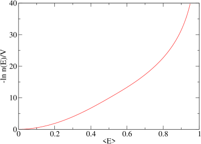
Figure 7: $-\ln n(E)/V$ as a function of plaquette energy[24].

Here we comment on the construction of the density of states. One can define the DOS for any other quantities. For instance, Gocksch[22] constructed the DOS for the complex phase. Ambjorn et al.[23] constructed the DOS for the number density in their factorization method. In these definitions of the DOS, simulation parameters $\beta$, $n_{f}$ and $m_{q}$ are absorbed in the DOS and the simulation parameters are not variable.

In the following we show results on $4^{4}$ lattices at isospin chemical potential $\mu_{V}$. The DOS $n(E)$ in eq.(19) can be obtained using the quenched data as[21]

$$-\frac{\ln n(E)}{V}=6\int^{E}_{0}dE^{\prime}\beta(E^{\prime})+const.$$ (24)

Figure 7 shows $-\ln n(E)/V$ as a function of plaquette energy $E$. The time consuming part of the method is the calculations of $\langle\det M(\mu)^{N_{f}/4}\rangle_{E}$ and $\langle O\det M(\mu)^{N_{f}/4}\rangle_{E}$ which contain the eigenvalue calculation. In order to generate configurations at fixed $E$ we used the over-relaxation method. At each $E$ we generated 100 configurations. Each configuration is separated by 100 over-relaxed updates. For each configuration we calculate eigenvalues and those eigenvalues are used to evaluate eqs.(22) and (23). Figure 8 shows $\langle\det M(\mu_{V})^{N_{f}/4}\rangle_{E}$ at $\mu_{V}=0.2$ and $m_{q}=0.025$ for various flavors as examples.

The isospin system has a positive measure and can be simulated with the standard Monte Carlo algorithm as R-algorithm[25]. Figure 9 compares the results from the DOS method with those from the R-algorithm. They are in good agreement with each other. Only a small difference is seen in the phase transition region.

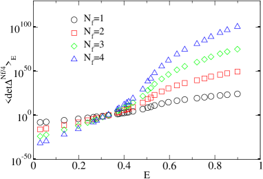
Figure 8: Microcanonical average of $\langle\det M(\mu_{V})^{N_{f}/4}\rangle_{E}$ at $\mu_{V}=0.2$ and $m_{q}=0.025$ as a function of $E$[24]

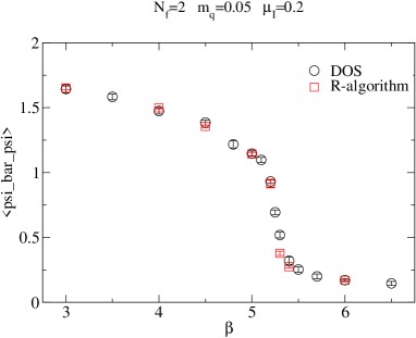
Figure 9: $\langle\bar{\psi}\psi\rangle$ for $n_{f}=2$ at $\mu_{V}=0.2$ and $m_{q}=0.05$[24].

Figure 10 shows $\langle\bar{\psi}\psi\rangle$ for different $n_{f}$ at $\mu_{V}=0.25$ and $m_{q}=0.05$. One can see that how $\beta_{c}$ changes as $n_{f}$, i.e. $\beta_{c}$ decreases as $n_{f}$ increases.

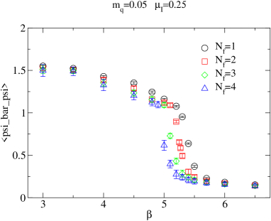
Figure 10: $\langle\bar{\psi}\psi\rangle$ for different $n_{f}$ at $\mu_{V}=0.25$ and $m_{q}=0.05$[24].

In the DOS method one may take various combinations of parameters. Let us consider the case of $n_{f}=1+1$ with non-degenerate quark masses $m_{1}$ and $m_{2}$. In this case one must calculate the following microcanonical averages:

$$\langle|\det\Delta(m_{1})|^{N_{f}/4}|\det\Delta(m_{2})|^{N_{f}/4}\rangle_{E},$$ (25)

$$\langle\bar{\psi}\psi(m_{i=1,2})|\det\Delta(m_{1})|^{N_{f}/4}|\det\Delta(m_{2})|^{N_{f}/4}\rangle_{E}.$$ (26)

Since the eigenvalues are stored, it is easy to calculate these microcanonical averages. On the other hand, in the conventional algorithm as R-algorithm, it is not easy to simulate the non-degenerate system since one needs a different program to perform the simulation. Figure 11(left) shows $\langle\bar{\psi}\psi\rangle$ for $n_{f}=1+1$ with different quark masses ( $m_{1}=0.05$ and $m_{2}=0.025$ ) at $\mu_{V}=0.2$.

Similarly one can also consider non-degenerate isospin chemical potentials $\mu_{1}$ and $\mu_{2}$. In this case one calculates

$$\langle|\det\Delta(\mu_{1})|^{N_{f}/4}|\det\Delta(\mu_{2})|^{N_{f}/4}\rangle_{E},$$ (27)

$$\langle\bar{\psi}\psi(\mu_{i=1,2})|\det\Delta(\mu_{1})|^{N_{f}/4}|\det\Delta(\mu_{2})|^{N_{f}/4}\rangle_{E}.$$ (28)

Figure 11(right) shows $\langle\bar{\psi}\psi\rangle$ for $n_{f}=1+1$ with different isospin chemical potentials ( $\mu_{1}=0.2$ and $\mu_{2}=0.3$ ) at $m_{q}=0.025$.

     

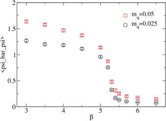
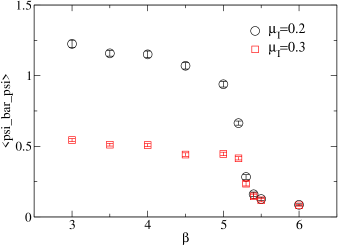
Figure 11: $\langle\bar{\psi}\psi(m_{q},\mu_{V})\rangle$ for $N_{f}=1+1$ at $\mu_{V}=0.2$ with different quark masses, ($m_{q}=0.05$ and $0.025$)(left), and at $m_{q}=0.025$ with different chemical potentials ($\mu_{V}$=0.2 and 0.3)[24].

In the DOS method one can easily obtain results for various parameters without making independent simulations. Thus the DOS method is considered to be useful to explore a wide parameter space. On the other hand, the eigenvalue calculations are computationally difficult on large lattices. Therefore the application of the DOS method might be limited on small lattices.

References

- [1] For recent reviews, see e.g., S. Muroya, A. Nakamura, C. Nonaka and T. Takaishi, Prog. Theor. Phys. 110 (2003) 615 [arXiv:hep-lat/0306031]; S. D. Katz, arXiv:hep-lat/0310051.
- [2] S. Choe et al. [QCD-TARO Collaboration], Nucl. Phys. Proc. Suppl. 106 (2002) 462 [arXiv:hep-lat/0110223].
- [3] S. Choe et al., Phys. Rev. D 65 (2002) 054501; Nucl. Phys. A 698 (2002) 395.
- [4] S.Gottlieb et al., \PRD38,1988,2888
- [5] R. V. Gavai and S. Gupta, Phys. Rev. D 68 (2003) 034506 [arXiv:hep-lat/0303013].
- [6] C. R. Allton, S. Ejiri, S. J. Hands, O. Kaczmarek, F. Karsch, E. Laermann and C. Schmidt, Phys. Rev. D 68 (2003) 014507 [arXiv:hep-lat/0305007].
- [7] S.Choe, Y.Liu, A.Nakamura and T.Takaishi, in preparation
- [8] O. Miyamura, S. Choe, Y. Liu, T. Takaishi and A. Nakamura, Phys. Rev. D 66 (2002) 077502 [arXiv:hep-lat/0204013].
- [9] C. R. Allton et al., Phys. Rev. D 66 (2002) 074507 [arXiv:hep-lat/0204010]. For the full reweighting approach without Taylor expansion, see Z. Fodor and S. D. Katz, Phys. Lett. B 534 (2002) 87 [arXiv:hep-lat/0104001]; Z. Fodor and S. D. Katz, JHEP 0203 (2002) 014 [arXiv:hep-lat/0106002].
- [10] P. de Forcrand, S. Kim and T. Takaishi, Nucl. Phys. Proc. Suppl. 119 (2003) 541 [arXiv:hep-lat/0209126].
- [11] Y. Sasai, A. Nakamura and T. Takaishi, arXiv:hep-lat/0310046.
- [12] D. Toussaint, Nucl. Phys. Proc. Suppl. 17 (1990) 248.
- [13] A. Nakamura and T. Takaishi, arXiv:hep-lat/0310052.
- [14] J. B. Kogut and D. K. Sinclair, arXiv:hep-lat/0309042.
- [15] T. Takaishi, Phys. Rev. D 54 (1996) 1050.
- [16] T. Takaishi and P. de Forcrand, Phys. Lett. B 428 (1998) 157 [arXiv:hep-lat/9802019].
- [17] P. de Forcrand et al. [QCD-TARO Collaboration], Nucl. Phys. B 577 (2000) 263 [arXiv:hep-lat/9911033].
- [18] S.Sasai, A.Nakamura and T.Takaishi, in preparation
- [19] G.Bhanot, K.Bitar and R.Salvador, Phys. Lett. B187 (1987) 381; Phys. Lett. B188 (1987) 246; M.Karliner, S.R.Sharpe and Y.F.Chang, Nucl. Phys. B302 (1988) 204
- [20] V.Azcoiti, G. di Carlo and A.F.Grillo, Phys. Rev. Lett. 65 (1990) 2239
- [21] X. Q. Luo, Mod. Phys. Lett. A 16 (2001) 1615 [arXiv:hep-lat/0107013].
- [22] A. Gocksch, Phys. Rev. Lett. 61 (1988) 2054.
- [23] J. Ambjorn, K. N. Anagnostopoulos, J. Nishimura and J. J. M. Verbaarschot, JHEP 0210 (2002) 062 [arXiv:hep-lat/0208025].
- [24] T. Takaishi, Mod. Phys. Lett. A 19 (2004) 909 [arXiv:hep-lat/0312038].
- [25] S.Gottlieb, W.Liu, D.Toussaint, R.L.Renken and R.L.Sugar, Phys. Rev. D 35 (1987) 2531