UTHEP-486
UTCCS-P-1
April, 2004
Light hadron spectroscopy in two-flavor QCD with small sea quark masses

Abstract

We extend the study of the light hadron spectrum and the quark mass in two-flavor QCD to smaller sea quark mass, corresponding to $m_{PS}/m_{V}=0.60$–0.35. Numerical simulations are carried out using the RG-improved gauge action and the meanfield-improved clover quark action at $\beta=1.8$ ($a=0.2$ fm from $\rho$ meson mass). We observe that the light hadron spectrum for small sea quark mass does not follow the expectation from chiral extrapolations with quadratic functions made from the region of $m_{PS}/m_{V}=0.80$–0.55. Whereas fits with either polynomial or continuum chiral perturbation theory (ChPT) fails, the Wilson ChPT (WChPT) that includes $a^{2}$ effects associated with explicit chiral symmetry breaking successfully fits the whole data: In particular, WChPT correctly predicts the light quark mass spectrum from simulations for medium heavy quark mass, such as $m_{PS}/m_{V}\,\hbox to0.0pt{\lower 3.5pt\hbox{$\mathchar 0\relax\sim$}\hss}\raise 1.0pt\hbox{$>$}\,0.5$. Reanalyzing the previous data with the use of WChPT, we find the mean up and down quark mass being smaller than the previous result from quadratic chiral extrapolation by approximately 10%, $m_{ud}^{\overline{\rm MS}}(\mu=2~{}\mbox{GeV})=3.11(17)$ [MeV] in the continuum limit.

I Introduction

Recent years have witnessed steady progress in the lattice QCD calculation of the light hadron spectrum plenary_lattice . In the quenched approximation ignoring quark vacuum polarization effects, well-controlled chiral and continuum extrapolations enabled a calculation of hadron masses with an accuracy of 0.5–3% quench.CP-PACS . At the same time the study established a systematic deviation of the quenched light hadron spectrum from experiment by approximately 10%. We then have made an attempt of full QCD calculation that allows chiral and continuum extrapolations within a consistent set of simulations Spectrum.Nf2.CP-PACS . The deviations from experiment in the light hadron spectrum are significantly reduced and the light quark mass decreases by about 25% with the inclusion of dynamical $u$ and $d$ quarks. With currently available computer power and simulation algorithms, however, the sea quark mass that can be explored is far from the physical value and a long chiral extrapolation is involved to get to the physical $u$ and $d$ quark mass.

An attempt has been made to push down the simulation to a small quark mass corresponding to $m_{PS}/m_{V}\approx 0.3$ in full QCD with the Kogut-Susskind(staggered)-type quark action Spectrum.Nf2.MILC . The staggered action, however, poses a problem of flavor mixing, which would modify the hadron spectrum and its quark mass dependence near the chiral limit. The staggered action also suffers from ambiguities in hadron operators and has a potential problem of non-locality. The Wilson-type quark actions have the advantage of simplicity: they are local and respect flavor symmetry, but a larger computational cost limits the simulations to relatively large quark masses corresponding to $m_{PS}/m_{V}\,\hbox to0.0pt{\lower 3.5pt\hbox{$\mathchar 0\relax\sim$}\hss}\raise 1.0pt\hbox{$>$}\,0.6$ Spectrum.Nf2.SESAM ; Spectrum.Nf2.TchiL ; Spectrum.Nf2.SESAM-TchiL ; Spectrum.Nf2.UKQCD.csw176 ; Spectrum.Nf2.UKQCD ; Spectrum.Nf2.CP-PACS ; Spectrum.Nf2.QCDSF ; Spectrum.Nf2.JLQCD . An important problem is to examine whether chiral extrapolations from such a quark mass range lead to results viable in the chiral limit.

Chiral extrapolations are usually made with polynomials in the quark mass. The problem is that they are not consistent with the logarithmic singularity expected in the chiral limit. In reality, the physical quarks are not exactly massless and hence the polynomial extrapolation should in principle work. However, increasingly higher orders are needed should one wish to increase the accuracy of the extrapolation. It is compelling to estimate the systematic errors due to higher order contributions when the data are extrapolated using a low-order polynomial.

An alternative choice for chiral extrapolations is to incorporate chiral perturbation theory (ChPT) ChPT.Gasser . The present lattice data, however, are not quite consistent with the ChPT predictions. The high-statistics JLQCD simulation of two-flavor full QCD, using the plaquette gauge action and the $O(a)$-improved Wilson quark action at $\beta=5.2$ ($a=0.0887(11)$ fm; the spatial size $L\simeq 1.06$–1.77 fm), shows no signature for the logarithmic singularity in the pion mass and pion decay constant Spectrum.Nf2.JLQCD . A possible reason for the failure to find the chiral logarithm is that sea quark masses, corresponding to $m_{PS}/m_{V}=0.8$–0.6, are too large. Higher order corrections of ChPT may have to be included to describe the data, as suggested from a partially quenched analysis, which shows that $m_{PS}/m_{V}=0.4$–0.3 is required for the convergence of one-loop formula PQChPT.Sharpe ; PQChPT.Durr . Another possibility is explicit chiral symmetry breaking of the Wilson quark actions that may invalidate the ChPT formulae. Modifications due to finite lattice spacings may be needed for an analysis of data obtained on a coarse lattice.

Recently studies were made to adapt ChPT to the Wilson-type fermion at finite lattice spacings (WChPT)  WChPT.Sharpe ; WChPT.Rupak ; WChPT.Oliver ; WChPT.Sinya , with subtle differences in the order counting, and hence the resulting formulae for observables, among the authors. The work WChPT.Rupak assumes the $O(a)$ chiral symmetry breaking effects being smaller than those from the quark mass, and only the effects linear in lattice spacing are retained in the chiral Lagrangian. This contrasts to the authors of Refs. WChPT.Oliver ; WChPT.Sinya who include the $O(a^{2})$ effects in the chiral Lagrangian, however, with different order countings. In Ref. WChPT.Oliver the $O(a)$ terms are treated as being comparable to the quark mass term while the $O(a^{2})$ terms are assumed to be subleading: in this case, $O(a)$ effects are essentially absorbed into the redefinition of the quark mass in the one-loop formulae and the $O(a^{2})$ terms provide additional counter terms. In Ref. WChPT.Sinya , on the other hand, the terms of $O(a^{2})$ are kept at the leading order, because the existence of parity-broken phase and vanishing of pion mass depend on them in a critical way WChPT.Sharpe . The coefficients of chiral logarithm terms receive $O(a)$ contributions, and hence the logarithmic chiral behavior is modified at a finite lattice spacing. Similar attempts to include the $O(a^{2})$ flavor mixing for the staggered-type quark action were made in Refs. SChPT.Lee ; SChPT.Bernard ; SChPT.Aubin .

The qq+q collaboration qq+q applied the one-loop ChPT and WChPT with the prescription of Refs. WChPT.Rupak ; WChPT.Oliver to their data obtained at $m_{PS}/m_{V}=0.9$–0.5. Their simulations were made at coarse lattices of $a=0.19$ fm $(\beta=5.1)$ and $0.28$ fm $(\beta=4.68)$ using the plaquette gauge action and the unimproved Wilson quark action ($L\approx 3$ fm). They reported that their data are described by these formulae. However, their sea quark masses are not quite small, and, since large scaling violation is suspected with unimproved actions at coarse lattice spacings and lattice artifacts are suggested at strong couplings lattice_artifact.MILC , it should be demonstrated at weaker couplings in order that the discretization effects are actually under control. The UKQCD collaboration reported a result at $m_{PS}/m_{V}=0.44(2)$ obtained with the actions and the lattice spacing the same as those of JLQCD, with $L\approx 1.6$ fm Spectrum.Nf2.UKQCD_light . They indicated the pion decay constant to bend slightly downward at this quark mass, but further work is required for quantitative comparison with the ChPT predictions.

In this paper, we follow up on our previous two-flavor full QCD work Spectrum.Nf2.CP-PACS with an RG-improved gauge action and tadpole-improved $O(a)$-improved Wilson-clover quark action at $m_{PS}/m_{V}=0.80$–0.55 and attempt to lower the quark mass to give $m_{PS}/m_{V}$ down to 0.35. Since the computational costs grows rapidly toward the chiral limit, roughly proportional to $(m_{PS}/m_{V})^{-6}$ cost.Ukawa , we concentrate our effort on the coarsest lattice of $a\approx 0.2$ fm at $\beta=1.8$, while using improved actions.

Generation of configurations below $m_{PS}/m_{V}\approx 0.5$ demands technical improvements. The BiCGStab algorithm sometimes fails to converge, which we overcome by an improvement called BiCGStab(DS-$L$) BiCGStab_DSL ; BiCGStab_IDSL.Itoh . Another problem is the emergence of instabilities in the HMC molecular dynamics evolution spike.Jansen ; spike.UKQCD . This seems to be caused by very small eigenvalues of the Dirac operator, leading to the change of the molecular dynamics orbit from elliptic to hyperbolic. The only resolution at present is to reduce the time step size. In this manner, we generated 4000 trajectories at $m_{PS}/m_{V}\approx 0.6$, 0.5 and 0.4 and 1400 trajectories at the smallest quark mass of $m_{PS}/m_{V}\approx 0.35$ on a $12^{3}\times 24$ lattice with $L\approx 2.4$ fm. To examine the finite-size effect, we also generated 2000 trajectories at $m_{PS}/m_{V}\approx 0.6$ and 0.5 on a $16^{3}\times 24$ lattice with $L\approx 3.2$ fm.

We calculate the light hadron spectrum and the quark mass on these configurations, and examine the validity of the quadratic chiral extrapolations by comparing the extrapolations made in the previous work with our new data at smaller quark masses. It turns out that the new data are increasingly lower than the extrapolation toward a smaller sea quark mass. We then examine how our data compare with the WChPT formulae, and whether WChPT fits using only the previous data at large quark masses predict correctly the new small quark mass data. This serves as a test to verify the viability of WChPT and of chiral extrapolations.

Computing for the present work was made on the VPP5000/80 at the Information Processing Center of University of Tsukuba. We used 4 or 8 nodes, each node having the peak speed of 9.6 Gflops. The present simulation costed 0.119 Tflops$\cdot$years of computing time measured in terms of the peak speed.

This paper is organized as follows. We describe configuration generations in Sec. II. The method of measurement of hadron masses, decay constants, quark masses and the static quark potential is explained in Sec. III. The finite-size effects on hadron masses are also discussed in the same section. Sec. IV discusses chiral extrapolations with conventional polynomials, and those based on ChPT are presented in Sec. V. Our conclusion is given in Sec. VI. Preliminary results of these calculations were reported in Ref. Spectrum.Nf2.CPPACS.lat02.Namekawa .

II Simulation

For the gauge part we employ the RG improved action defined by

$$S_{g}=\frac{\beta}{6}\left\{c_{0}\sum_{x,\mu\nu}W_{\mu\nu}^{1\times 1}(x)+c_{1}\sum_{x,\mu\nu}W_{\mu\nu}^{1\times 2}(x)\right\}.$$ (1)

The coefficients $c_{0}=3.648$ of the $1\times 1$ Wilson loop and $c_{1}=-0.331$ of the $1\times 2$ Wilson loop are determined by an approximate renormalization group analysis RGaction . They satisfy the normalization condition $c_{0}+8c_{1}=1$, and $\beta=6/g^{2}$. For the quark part we use the clover quark action SWaction defined by

$$S_{q} = \sum_{x,y}\overline{q}_{x}D_{x,y}q_{y},$$ (2)

$$D_{x,y} = \delta_{xy}-\kappa\sum_{\mu}\left\{(1-\gamma_{\mu})U_{x,\mu}\delta_{x+\hat{\mu},y}+(1+\gamma_{\mu})U_{x,\mu}^{{\dagger}}\delta_{x,y+\hat{\mu}}\right\}-\,\delta_{xy}c_{\rm SW}\kappa\sum_{\mu<\nu}\sigma_{\mu\nu}F_{\mu\nu},$$ (3)

where $\kappa$ is the hopping parameter, $F_{\mu\nu}$ the standard clover-shaped lattice discretization of the field strength and $\sigma_{\mu\nu}=(i/2)[\gamma_{\mu},\gamma_{\nu}]$. For the clover coefficient we adopt a meanfield improved value $c_{\rm SW}=u_{0}^{-3}$ tadpole_improvement where

$$u_{0}=\left(W^{1\times 1}\right)^{1/4}=\left(1-0.8412\beta^{-1}\right)^{1/4},$$ (4)

using the plaquette $W^{1\times 1}$ calculated in one-loop perturbation theory RGaction . This choice is based on our observation that the one-loop calculation reproduces the measured values well Comparative.Nf2.CP-PACS .

Our simulation is performed at a single value of $\beta=1.8$ using two lattice sizes $12^{3}\times 24$ and $16^{3}\times 24$ to study finite size effects. The lattice spacing fixed from $m_{\rho}$ at the physical sea quark mass is 0.2 fm. We adopt four values of the sea quark mass corresponding to the hopping parameter $\kappa_{sea}=0.14585$, $0.14660$, $0.14705$ and $0.14720$. This choice covers $m_{PS}/m_{V}=0.60$–0.35, extending the four values $\kappa_{sea}=0.1409$, 0.1430, 0.1445, and 0.1464 corresponding to $m_{PS}/m_{V}=0.80$–0.55 studied in Ref. Spectrum.Nf2.CP-PACS . The simulation parameters are summarized in Table 1, where we also list the number of nodes (PE’s) employed and the CPU time per trajectory. Gauge configurations are generated using the Hybrid Monte Carlo (HMC) algorithm HMC.Duane ; HMC.Gottlieb . The trajectory length in each HMC step is fixed to unity. We use the leap-frog integration scheme for the molecular dynamics equation.

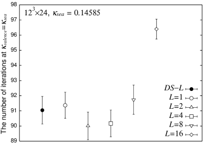
Figure 2: The number of iterations required with BiCGStab($L$) and BiCGStab(DS-$L$) for inversions of the quark matrix at $\kappa_{sea}=\kappa_{valence}=0.14585$ ($m_{PS}/m_{V}=0.60$) on $12^{3}\times 24$ lattice. Conventional BiCGStab corresponds to $L=1$.

The even/odd preconditioned BiCGStab BiCGStab is one of the most optimized algorithms for the Wilson quark matrix inversion to solve the equation $D_{xy}G_{y}=B_{x}$. However, BiCGStab sometimes fails to converge at small sea quark masses. While the CG algorithm is guaranteed to converge, it is time-consuming. We find that the BiCGStab($L$) algorithm BiCGStab_L.Sleijpen , which is an extension of BiCGStab to $L$-th order minimal residual polynomials, is more stable BiCGStab_IDSL.Itoh . Figure 1 illustrates for a very light valence quark mass corresponding to $m_{PS}/m_{V}=0.27$ that the BiCGStab($L$), while not convergent for $L=1$ and 2, succeeds to find the solution for $L=4$. In practice, however, too large $L$ also frequently introduces another instability from possible loss of conjugacy among the $L$ vectors. The optimum value of $L$ depends on simulation parameters. To avoid a tuning of $L$ at each simulation point, we employ the BiCGStab(DS-$L$) algorithm BiCGStab_DSL . This is a modified BiCGStab($L$) in which a candidate of the optimum $L$ is dynamically selected. We find that BiCGStab(DS-$L$) is much more robust than the original BiCGStab at small quark masses. We also find that, at large quark masses where the conventional BiCGStab converges, the computer time required for BiCGStab(DS-$L$) is comparable. See Fig. 2. Therefore, we adopt BiCGStab(DS-$L$) at all values of our sea quark masses.

We employ the stopping condition $||DG-B||<\Delta$ in HMC. The value of $\Delta$ in the evaluation of the fermionic force is chosen so that the reversibility over unit length is satisfied to a relative precision of order $10^{-8}$ or smaller for the Hamiltonian,

$$|\Delta H|=|H_{reversed}-H_{0}|,$$ (5)

where $H_{reversed}$ is the value of the Hamiltonian obtained by integrating to $t=1$ and integrating back to $t=0$. We also check the reversibility violation in the link variable,

$$|\Delta U|=\sqrt{\sum_{n,\mu,a,b}U_{\mu,a,b}^{reversed}(n)-U_{\mu,a,b}^{0}(n)},$$ (6)

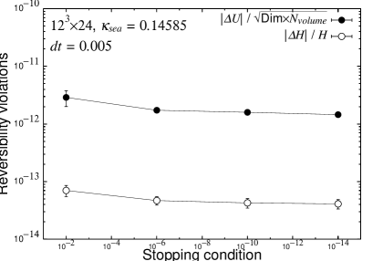
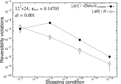
Figure 3: Reversibility violation at large sea quark mass of $\kappa_{sea}=0.14585$ ($m_{PS}/m_{V}=0.60$) (left panel) and small sea quark mass of $\kappa_{sea}=0.14705$ ($m_{PS}/m_{V}=0.40$) (right panel) on $12^{3}\times 24$ lattice.

where the sum is taken over all sites $n$, colors $a,b$ and the link directions $\mu$. We illustrate our check in Fig. 3, where results at $\kappa_{sea}=0.14585$ and $\kappa_{sea}=0.14705$ on 20 thermalized configurations separated by 100 trajectories are shown. When the sea quark mass is large ($\kappa_{sea}=0.14585,m_{PS}/m_{V}=0.6$), the violation does not show any clear dependence on the stopping condition. For small sea quark mass ($\kappa_{sea}=0.14705$, $m_{PS}/m_{V}=0.4$), however, it depends on the stopping condition significantly. We must be careful with the choice of the stopping condition at small sea quark mass. We use a stricter stopping condition in the calculation of the Hamiltonian in the Metropolis accept/reject test. Table 1 shows our choice of $\Delta$ together with the average number, $N_{inv}$, of the BiCGStab(DS-$L$) iterations in the quark matrix inversion for the force calculation.

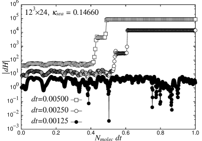
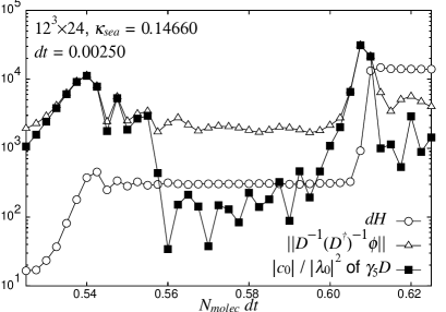
Figure 4: Effect of the molecular dynamics step size $dt$ on the appearance of spikes in $dH\equiv H_{trial}-H_{0}$ at $\kappa_{sea}=0.14660$ ($m_{PS}/m_{V}=0.50$) on $12^{3}\times 24$ lattice (left panel). The right panel is an enlargement around the spikes in the case of $dt=0.0025$. $||D^{-1}(D^{\dagger})^{-1}\phi||$ with the Wilson-clover operator $D$ and the pseudofermion field $\phi$ as well as the corresponding contribution with the smallest eigenvalue $\lambda_{0}$ and its overlap $c_{0}\equiv(x_{0},\phi)$ for $\gamma_{5}D$ are also plotted, where $x_{i}$ is an eigenfunction of $\gamma_{5}D$ such that $\phi=\sum_{i}c_{i}x_{i}$.

In the course of configuration generation by the HMC algorithm, we sometimes encountered extremely large values of $dH\equiv H_{trial}-H_{0}$, the difference of the trial and starting Hamiltonians. Similar experiences have been reported by other groups spike.Jansen ; spike.UKQCD . Empirically this phenomenon occurs more frequently for smaller sea quark masses at a fixed step size, and can be suppressed by decreasing the step size. A typical example is shown in Fig. 4. In our runs we employ a step size $dt$ small enough for this purpose. As a consequence our runs have a rather high acceptance 80–90%. It is possible that this phenomenon is connected to the appearance of very small eigenvalues of the Wilson-clover operator toward small quark masses. In the right panel of Fig. 4, we show the norm $||D^{-1}(D^{\dagger})^{-1}\phi||$ (triangles) and the contribution of the smallest eigenvalue of $\gamma_{5}D$ to the norm (filled squares). We observe that the jump of $dH$ (open circles) is associated with a peak of the norm, and that the peak is saturated by the contribution of the smallest eigenvalue. We suspect that such small eigenvalues cause some modes of the HMC molecular dynamics evolution to change its character from elliptic to hyperbolic, leading to divergence of the Hamiltonian. We defer a further study of this problem to future publications.

We accumulate 4000 HMC trajectories at $\kappa_{sea}=0.14585$, $0.14660$ and $0.14705$ and 1400 trajectories at $\kappa_{sea}=0.14720$ on the $12^{3}\times 24$ lattice. We also accumulate 2000 trajectories at $\kappa_{sea}=0.14585$ and $0.14660$ on the $16^{3}\times 24$ lattice. Measurements of light hadron masses and the static quark potential are carried out at every 5 trajectories.

III Measurement

III.1 Hadron masses

The meson operators are defined by

$$M(x)=\bar{q}^{(f)}(x)\Gamma q^{(g)}(x),\hskip 14.22636pt\Gamma=I,\gamma_{5},\gamma_{\mu},\gamma_{5}\gamma_{\mu},$$ (7)

where $f$ and $g$ are flavor indices and $x$ is the coordinates on the lattice. The octet baryon operator is defined as

$$O^{fgh}(x)=\epsilon^{abc}\left(q^{(f)a}(x){}^{T}C\gamma_{5}q^{(g)b}(x)\right)q^{(h)c}(x),$$ (8)

where $a,b,c$ are color indices and $C=\gamma_{4}\gamma_{2}$ is the charge conjugation matrix. Decuplet baryon correlators are calculated using an operator defined by

$$D^{fgh}_{\mu}(x)=\epsilon^{abc}\left(q^{(f)a}(x){}^{T}C\gamma_{\mu}q^{(g)b}(x)\right)q^{(h)c}(x).$$ (9)

For each configuration quark propagators are calculated with a point and a smeared source. For the smeared source, we fix the gauge configuration to the Coulomb gauge and use an exponential smearing function $\psi(r)=A\exp(-Br)$ for $r>0$ with $\psi(0)=1$. We chose $A=1.25$ and $B=0.50$ as in our previous study Spectrum.Nf2.CP-PACS . In order to reduce the statistical fluctuation of hadron correlators, we repeat the measurement for two choices of the location of the hadron source, $t_{src}=1$ and $N_{t}/2+1(=13)$ and take the average over the two Spectrum.Nf2.JLQCD :

$$\frac{1}{2}\left(\left\langle H(t_{src}+t)H(t_{src})^{\dagger}\right\rangle_{t_{src}=1}+\left\langle H(t_{src}+t)H(t_{src})^{\dagger}\right\rangle_{t_{src}=N_{t}/2+1}\right).$$ (10)

This procedure reduces the statistical error of hadron correlators typically by 30 to 40%, which suggests that the statistics are increased effectively by a factor of 1.7 to 2. For further reduction of the statistical fluctuation, we take the average over three polarization states for vector mesons, two spin states for octet baryons and four spin states for decuplet baryons.

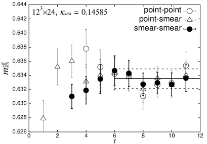
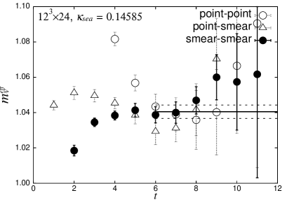
Figure 5: Effective masses of pseudoscalar (left panel) and vector meson (right panel) at $\kappa_{sea}=0.14585$ ($m_{PS}/m_{V}=0.60$) on $12^{3}\times 24$ lattice.

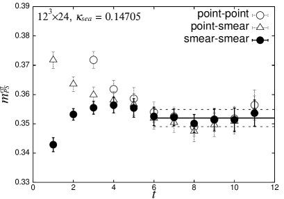
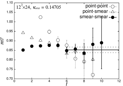
Figure 6: Effective masses of pseudoscalar (left panel) and vector meson (right panel) at $\kappa_{sea}=0.14705$ ($m_{PS}/m_{V}=0.40$) on $12^{3}\times 24$ lattice.

Figures 5 and 6 illustrate the quality of effective mass plots. For mesons, an acceptable plateau of the effective mass is obtained from hadron correlators with the point sink and the doubly smeared source. Signals are much worse for baryons.

We carry out $\chi^{2}$ fits to hadron correlators, taking account of correlations among different time slices. A single hyperbolic cosine form is assumed for mesons, and a single exponential form for baryons. We set the lower cut of the fitting range as $t_{min}=6$ for mesons and $t_{min}=5$ for baryons, which is determined by inspecting stability of the resulting mass. The upper cut ($t_{max}$) dependence of the fit is small and, therefore, we fix $t_{max}$ to $N_{t}/2$ for all hadrons. Our choice of fit ranges and the detailed results of hadron masses are given in tables of Appendix A. Statistical errors of hadron masses are estimated with the jack-knife procedure. We adopt the bin size of 100 trajectories from an analysis of the bin size dependence of errors as discussed below in Sec. III.5.

III.2 Quark masses

We calculate the mean up and down quark mass through both vector and axial-vector Ward identities. The two types of quark masses, denoted by $m_{VWI}$ and $m_{AWI}$ respectively, differ at finite lattice spacings because of explicit violation of chiral symmetry by the Wilson term.

A bare VWI quark mass is defined by

$$m_{quark}^{VWI}=\frac{1}{2}\left(\frac{1}{\kappa}-\frac{1}{\kappa_{c}}\right).$$ (11)

The critical hopping parameter $\kappa_{c}$ is determined by chiral extrapolations as discussed in Sec. IV and V. A bare AWI quark mass is calculated using the fourth component of the improved axial-vector current

$$A_{4}^{\rm imp}=A_{4}+c_{A}\partial_{4}P,$$ (12)

where $P$ is the pseudoscalar meson operator, Eq. (7) with $\Gamma=\gamma_{5}$, and $\partial_{4}$ is the symmetric lattice derivative. Then, $m_{quark}^{AWI}$ is obtained through

$$m_{quark}^{AWI}=\frac{m_{PS}C_{A}^{s}}{2C_{P}^{s}}.$$ (13)

The amplitudes $C_{A}^{s}$ and $C_{P}^{s}$ are calculated as follows. We determine the pseudoscalar meson mass $m_{PS}$ and $C_{P}^{s}$ by

$$\langle P^{l}(t)P^{s}(0)^{\dagger}\rangle=C_{P}^{s}\left[\exp(-m_{PS}t)+\exp(-m_{PS}(L_{t}-t))\right],$$ (14)

where the superscripts $l$ and $s$ distinguish local and smeared operators. Keeping $m_{PS}$ fixed, we extract $C_{A}^{s}$ from

$$\langle A_{4}^{{\rm imp},l}(t)P^{s}(0)^{\dagger}\rangle=C_{A}^{s}\left[\exp(-m_{PS}t)-\exp(-m_{PS}(L_{t}-t))\right].$$ (15)

The renormalized quark masses in the $\overline{\mbox{MS}}$ scheme at 2 GeV are obtained as follows. The VWI up and down quark mass

$$m_{ud}^{VWI}=\frac{1}{2}\left(\frac{1}{\kappa_{ud}}-\frac{1}{\kappa_{c}}\right),$$ (16)

with $\kappa_{ud}$ the hopping parameter at the physical point, is renormalized using one-loop renormalization constants and improvement coefficients at $\mu=1/a$:

$$m_{ud}^{VWI,\overline{\rm MS}}(\mu=1/a)=Z_{m}\left(1+b_{m}\frac{m_{ud}^{VWI}}{u_{0}}\right)\frac{m_{ud}^{VWI}}{u_{0}}.$$ (17)

Similarly the renormalized AWI quark mass is obtained by

$$m_{ud}^{AWI,\overline{\rm MS}}(\mu=1/a)=\frac{Z_{A}\left(1+b_{A}\frac{m_{ud}^{VWI}}{u_{0}}\right)}{Z_{P}\left(1+b_{P}\frac{m_{ud}^{VWI}}{u_{0}}\right)}m_{ud}^{AWI},$$ (18)

where $m_{ud}^{AWI}$ is the value of $m_{quark}^{AWI}$ extrapolated to $\kappa_{ud}$. The determination of $\kappa_{ud}$ is discussed in Sec. IV and V. Since non-perturbative values for the renormalization coefficient $Z_{A}$ and the improvement parameters $c_{A}$, $b_{A}$ etc. are not available for our combination of actions in two-flavor QCD, we adopt one-loop perturbative values calculated in Refs. Z_factors.Sinya1 ; Z_factors.Sinya2 improved with the tadpole procedure using $u_{0}$ given in Eq.(4). The $\overline{\mbox{MS}}$ quark masses at $\mu=1/a$ are evolved to $\mu=2$ GeV using the four-loop beta function Run_factor.Chetrykin ; Run_factor.Vermaseren .

III.3 Decay constants

The pseudoscalar meson decay constant is calculated by

$$f_{PS}=2\kappa u_{0}Z_{A}\left(1+b_{A}\frac{m_{quark}^{VWI}}{u_{0}}\right)\frac{C_{A}^{s}}{C_{P}^{s}}\sqrt{\frac{C_{P}^{l}}{m_{PS}}},$$ (19)

where $C_{P}^{l}$ is determined by

$$\langle P^{l}(t)P^{l}(0)^{\dagger}\rangle=C_{P}^{l}\left[\exp(-m_{PS}t)+\exp(-m_{PS}(L_{t}-t))\right],$$ (20)

keeping $m_{PS}$ fixed to the value from $\langle P^{l}(t)P^{s}(0)^{\dagger}\rangle$.

The vector meson decay constant $f_{V}$ is defined as

$$\langle 0|V_{i}|{V}\rangle=\epsilon_{i}f_{V}m_{V},$$ (21)

where $\epsilon_{i}$ is a polarization vector. The procedure to obtain the vector meson decay constant is parallel to that for $f_{PS}$. The vector meson correlator with a smeared source is fitted with

$$\langle V^{l}(t)V^{s}(0)^{\dagger}\rangle=C_{V}^{s}\left[\exp(-m_{V}t)+\exp(-m_{V}(L_{t}-t))\right],$$ (22)

which determines $m_{V}$ and $C_{V}^{s}$. Using $m_{V}$ as an input we fit the correlator

$$\langle V^{l}(t)V^{l}(0)^{\dagger}\rangle=C_{V}^{l}\left[\exp(-m_{V}t)+\exp(-m_{V}(L_{t}-t))\right],$$ (23)

where the amplitude $C_{V}^{l}$ is the only fit parameter. A renormalized vector meson decay constant is then obtained through

$$f_{V}=2\kappa u_{0}Z_{V}\left(1+b_{V}\frac{m_{VWI}}{u_{0}}\right)\sqrt{\frac{C_{V}^{l}}{m_{V}}},$$ (24)

where we also use one-loop perturbative values for $Z_{V}$ and $b_{V}$ Z_factors.Sinya1 ; Z_factors.Sinya2 . We do not include the improvement term $c_{V}\tilde{\partial}_{\nu}T_{n\mu\nu}$ because the corresponding correlator is not measured.

III.4 Static quark potential

We calculate the static quark potential $V(r)$ from the temporal Wilson loops $W(r,t)$

$$W(r,t)=C(r)\exp\left(-V(r)t\right).$$ (25)

We apply the smearing procedure of Ref. Potential.Bali . The number of smearing steps is fixed to its optimum value $N_{opt}=2$ at which the overlap to the ground state $C(r)$ takes the largest value. Let us define an effective potential

$$V_{eff}(r,t)=\log\left[W(r,t)/W(r,t+1)\right].$$ (26)

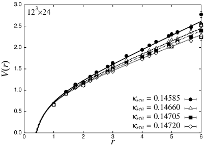
Figure 8: Static quark potentials at $\kappa_{sea}=0.14585,0.14660,0.14705$ and $0.14720$ correspond to $m_{PS}/m_{V}=0.60,0.50,0.40$ and $0.35$ on $12^{3}\times 24$ lattice.

Examples of $V_{eff}$ are plotted in Fig. 7, from which we take the lower cut of $t_{min}=2$. As shown in Fig. 8, we do not observe any clear indication of the string breaking. Therefore, we carry out a correlated fit to $V(r)=V_{eff}(r,t_{min})$ with

$$V(r)=V_{0}-\frac{\alpha}{r}+\sigma r.$$ (27)

Here we do not include the lattice correction to the Coulomb term calculated perturbatively from one lattice-gluon exchange diagram deltaV , since rotational symmetry is well restored for our RG-improved action. The Sommer scale $r_{0}$ is defined through r_0

$$r_{0}^{2}\left.\frac{dV(r)}{dr}\right|_{r=r_{0}}=1.65.$$ (28)

We determine $r_{0}$ from the parameterization of the potential $V(r)$:

$$r_{0}=\sqrt{\frac{1.65-\alpha}{\sigma}}.$$ (29)

The lower cut of the fit range in Eq. (27) is determined as $r_{min}=\sqrt{2}$ from inspection of the $r_{min}$ dependence of $r_{0}$. With $r_{min}<\sqrt{2}$, $\chi^{2}/{dof}$ takes an unacceptably large value, while $\alpha$ becomes ill-determined with $r_{min}>\sqrt{3}$. On the other hand, the $r_{max}$ dependence of $r_{0}$ is mild. Therefore, we fix $r_{max}$ to $N_{s}/2$. We estimate the systematic error of the fit as follows. The fit of Eq. (27) is repeated with other choices of the range: $t_{min}=3$ or $r_{min}=\sqrt{3}$. The variations in the resulting parameters and $r_{0}$ are taken as systematic errors. The parameters in Eq. (27) and $r_{0}$ are presented in Table 2.

III.5 Autocorrelation

The autocorrelation in our data is studied by the cumulative autocorrelation time

$$\tau^{cum}_{\mathcal{O}}(\Delta t_{max})=\frac{1}{2}+\sum_{\Delta t=1}^{\Delta t_{max}}\rho_{\mathcal{O}}(\Delta t),$$ (30)

where $\rho_{\mathcal{O}}(t)$ is the autocorrelation function

$$\rho_{\mathcal{O}}(\Delta t)=\frac{\Gamma_{\mathcal{O}}(\Delta t)}{\Gamma_{\mathcal{O}}(0)},\\ ~{}~{}~{}\Gamma_{\mathcal{O}}(\Delta t)=\langle\left(\mathcal{O}(t)-\langle\mathcal{O}\rangle\right)\left(\mathcal{O}(t+\Delta t)-\langle\mathcal{O}\rangle\right)\rangle.$$ (31)

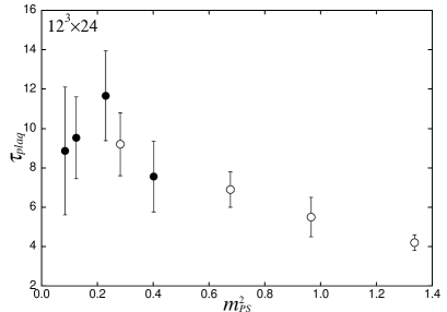
Figure 10: Sea quark mass dependence of the cumulative autocorrelation time of plaquette on $12^{3}\times 24$ lattice. Open symbols are the results obtained in our previous study Spectrum.Nf2.CP-PACS .

A conventional choice for $\Delta t_{max}$ is the first point where $\rho_{\mathcal{O}}$ vanishes because $\rho_{\mathcal{O}}$ should be positive when the statistics are sufficiently high. We take $\Delta t_{max}=50$ from the plaquette shown in Fig. 9. In Table 3, we give $\tau^{cum}_{\cal O}$ for (i) the plaquette which is measured at every trajectory, (ii) the pseudoscalar meson propagators at $t=N_{t}/4$, and (iii) the temporal Wilson loop with $(r,t)=(2,2)$. Fig. 10 shows the autocorrelation time for the plaquette. Combining the previous (open circles) and the new (filled circles) data, we observe a trend of increase for smaller quark masses. A sharp rise expected toward the chiral limit, however, is not seen. Our statistics may not be sufficient to estimate autocorrelation times reliably near the chiral limit.

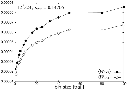
Figure 11: Bin size dependence of jack-knife error of pseudoscalar meson mass (left panel), and plaquette and rectangular loop (right panel) at $\kappa_{sea}=0.14705$ ($m_{PS}/m_{V}=0.40$) on $12^{3}\times 24$ lattice.

The bin size dependence of the jack-knife errors of hadron masses and Wilson loops is exhibited in Figs. 11. The jack-knife errors reach plateaus at bin size of 50–100 trajectories. The situation is similar on $16^{3}\times 24$. Therefore, we take the bin size of 100 trajectories in the error analysis.

III.6 Finite-size effects

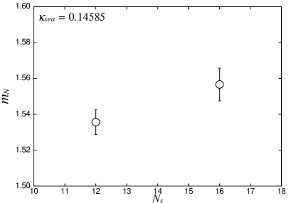
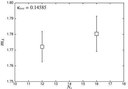
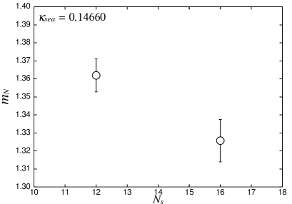
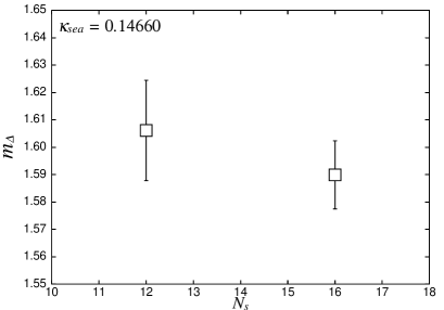
Figure 14: Volume dependence of octet (left panel) and decuplet baryon masses (right panel) at $\kappa_{sea}=0.14585$ ($m_{PS}/m_{V}=0.60$) and $\kappa_{sea}=0.14660$ ($m_{PS}/m_{V}=0.50$).

In Figs. 12 and 13, we present meson and AWI quark masses as a function of the spatial volume. The results obtained on $12^{3}\times 24$ and $16^{3}\times 24$ lattices are mutually consistent within errors. For baryons, there may be some indication in our data at $m_{PS}/m_{V}=0.50$ ($\kappa_{sea}=0.14660$) that the light baryon masses $m_{N}$ and $m_{\Delta}$ decrease by 1–3% (0.8–3.1$\sigma$) as shown in Fig. 14. The effect is only around 2$\sigma$, and higher statistics are needed to confirm if the difference can be attributed to finite-size effects. Finite-size effects in $r_{0}$ are expected to be much smaller than those in hadron masses. Our results in Fig. 15 confirm this. In the following analysis, we use data obtained on the $12^{3}\times 24$ lattice.

IV Chiral extrapolation with polynomials

Extrapolation of the lattice simulation data to physical values requires some parameterization of the data as functions of the quark mass. In this section, we employ polynomials in quark masses. We work with the two data sets, the one obtained in the previous work that covers $m_{PS}/m_{V}=0.80$–0.55 (the large quark mass data set), and the other obtained in the present work that covers $m_{PS}/m_{V}=0.60$–0.35 (the small quark mass data set), and with the combined data set of the two. For the large mass data set we borrow the fit from the previous work.

We fit hadron masses in lattice units rather than those normalized by $r_{0}$. With our choice of the improved actions, $r_{0}$ exhibits only a mild sea quark mass dependence as shown below in Sec. IV.3, and hence introducing $r_{0}$ does not change convergence of chiral extrapolations. From practical side, $r_{0}$ suffers from a large systematic error on coarse lattices with $a=0.2$ fm. Hence fits become less constraining if hadron masses are normalized by $r_{0}$.

IV.1 Pseudoscalar meson mass and AWI quark mass

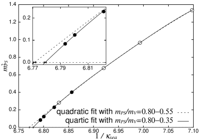
Figure 16: Chiral extrapolation of pseudoscalar meson mass. Open symbols show the results obtained in the previous calculation Spectrum.Nf2.CP-PACS and filled symbols are our new results. Lines are polynomial fits as explained in the figure.

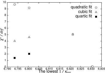
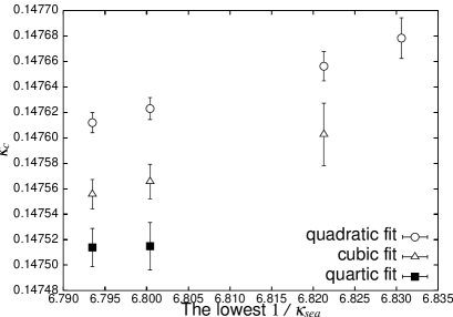
Figure 17: Dependence of $\chi^{2}/dof$ on the fitting range and order of the fitting polynomial (left panel), and that of the critical hopping parameter (right panel) for pseudoscalar meson mass. Symbols are placed at the value of $1/\kappa_{sea}$ corresponding to the lowest fitting range, which is changed as shown in the figure, while the highest is fixed to $\kappa_{sea}=0.1409$ ($m_{PS}/m_{V}=0.80$). Quadratic, cubic and quartic forms as a function of VWI quark mass are tested.

A quadratic form fitted well our previous lattice data of the pseudoscalar meson mass with a reasonable $\chi^{2}/dof\sim 1$ Spectrum.Nf2.CP-PACS . As shown in Fig. 16, however, our new data at small sea quark masses deviate significantly from the quadratic fit. Inclusion of the small quark mass data set in the quadratic fit rapidly increases $\chi^{2}/dof$ to $\sim 10$. In addition, the determination of the critical hopping parameter $\kappa_{c}$ becomes unstable as shown in Fig. 17. A reasonable $\chi^{2}/dof$ and a stable fit are achieved only when we extend the polynomial to quartic,

$$m_{PS}^{2}=B^{PS}m_{quark}^{VWI}+C^{PS}(m_{quark}^{VWI})^{2}+D^{PS}(m_{quark}^{VWI})^{3}+E^{PS}(m_{quark}^{VWI})^{4},$$ (32)

where $m_{quark}^{VWI}$ is given in Eq.(11) and $\kappa_{c}$ is taken as a fit parameter. The quartic polynomial provides the best fit among our tests varying the order of polynomials.

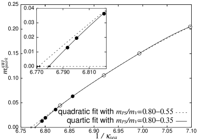
Figure 18: Chiral extrapolation of AWI quark masses. Open symbols show the results obtained in the previous calculation Spectrum.Nf2.CP-PACS . Lines are polynomial fits as explained in the figure.

Since $m_{PS}^{2}$ may be affected by the logarithmic singularity of ChPT, we examine the convergence of extrapolations, i.e., whether it depends on the order of polynomials, using $m_{quark}^{AWI}$ that has no logarithmic singularities. Along with the case of $m_{PS}^{2}$, the new data at small quark masses deviate from the quadratic fit obtained from the large quark mass data, as depicted in Fig. 18. We fit $m_{quark}^{AWI}$ by

$$m_{quark}^{AWI}=B^{AWI}m_{quark}^{VWI}+C^{AWI}(m_{quark}^{VWI})^{2}+D^{AWI}(m_{quark}^{VWI})^{3}+E^{AWI}(m_{quark}^{VWI})^{4}.$$ (33)

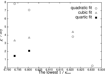
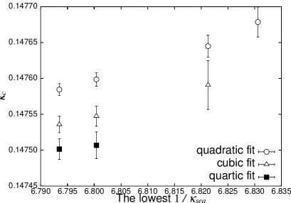
Figure 19: Dependence of $\chi^{2}/dof$ on the fitting range and order of the fitting polynomial (left panel), and that of the critical hopping parameter (right panel) for AWI quark mass. Symbols are placed at the value of $1/\kappa_{sea}$ corresponding to the lowest fitting range, which is changed as shown in the figure, while the highest is fixed to $\kappa_{sea}=0.1409$ ($m_{PS}/m_{V}=0.80$). Quadratic, cubic and quartic forms as a function of VWI quark mass are tested.

The fit range and order dependence are given in Fig. 19. $(m_{quark}^{VWI})^{4}$ terms are needed again to obtain a reasonable $\chi^{2}/dof$.

We find that $\kappa_{c}$ determined from $m_{PS}^{2}$ agrees with that from $m_{quark}^{AWI}$ within errors. Hence we simultaneously fit $m_{PS}^{2}$ and $m_{quark}^{AWI}$ to determine $\kappa_{c}$. The resulting independent and simultaneous fits to $m_{PS}^{2}$ and $m_{quark}^{AWI}$ are presented in Tables 4 and 5, respectively. The difference in mass from the fits including $(m_{quark}^{VWI})^{5}$ is taken as systematic errors. These errors represent only uncertainties within polynomial extrapolations. As shown in Sec. V.2, WChPT fits sometimes lead to values beyond these systematic errors.

IV.2 Vector meson mass

We fit vector meson mass with a cubic polynomial in $m_{PS}^{2}$,

$$m_{V}=A^{V}+B^{V}m_{PS}^{2}+D^{V}m_{PS}^{4}+F^{V}m_{PS}^{6}$$ (34)

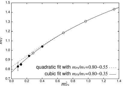
Figure 20: Chiral extrapolation of vector meson mass in terms of pseudoscalar meson mass. Open symbols show the results obtained in the previous calculation Spectrum.Nf2.CP-PACS .

with the results shown in Fig. 20 and Table 6. As in the case of $m_{PS}^{2}$ and $m_{quark}^{AWI}$, systematic deviations from the previous fit are observed, although the difference (7% or 3.6$\sigma$ in the chiral limit) is smaller. Inclusion of terms $m_{PS}^{4}$ and $m_{PS}^{6}$ gives a good fit with a satisfactory $Q$. We estimate the systematic error from higher order terms by the difference from the fit with $m_{PS}^{8}$ term.

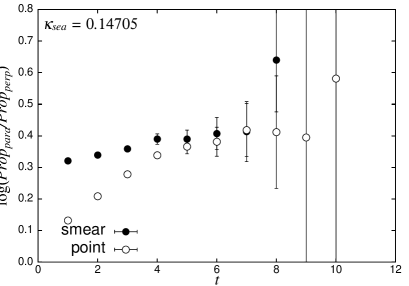
Figure 21: Ratio of vector meson correlators with momentum $2\pi/L$ and the polarization parallel and perpendicular to it.

The effects of vector meson decays are not considered in the fit. If a vector meson decays into two pseudoscalar mesons, a vector meson with the momentum $p=2\pi/L$ will take a different energy depending on whether it is polarized parallel or perpendicular to the momentum direction, because of mixing of one vector meson state and two pseudoscalar meson state rho_decay.MILC ; rho_decay.UKQCD . We find no indication of vector meson decays as shown in Fig. 21. Our sea quark masses and the lattice size do not seem to be enough to allow the decay.

IV.3 Decay constants, baryon masses and Sommer scale

Chiral extrapolations are carried out for pseudoscalar and vector meson decay constants and octet and decuplet baryon masses using cubic polynomials in $m_{PS}^{2}$,

$$f_{PS,V}=A^{f_{PS},f_{V}}+B^{f_{PS},f_{V}}m_{PS}^{2}+D^{f_{PS},f_{V}}m_{PS}^{4}+F^{f_{PS},f_{V}}m_{PS}^{6},$$ (35)

$$m_{oct,dec}=A^{oct,dec}+B^{oct,dec}m_{PS}^{2}+D^{oct,dec}m_{PS}^{4}+F^{oct,dec}m_{PS}^{6}.$$ (36)

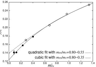
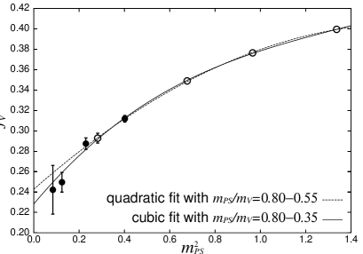
Figure 22: Chiral extrapolation of pseudoscalar (left panel) and vector (right panel) meson decay constants. Open symbols show the results obtained in the previous calculation Spectrum.Nf2.CP-PACS .

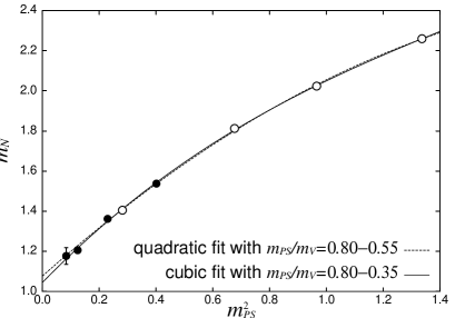
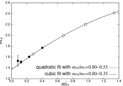
Figure 23: Chiral extrapolation of octet (left panel) and decuplet (right panel) baryon masses. Open symbols are the results in our previous study Spectrum.Nf2.CP-PACS .

The results are presented in Figs. 22 and 23 and Tables 7 and 8. While the decay constants show clear deviations from the previous fit, baryon masses are almost on the fit. We gather that the latter is an accidental effect that is caused by a compensation of the downward shift of baryon masses expected toward a small quark mass with an upward finite-size shift caused by somewhat too small a lattice ($L=2.4$ fm) for baryons (see Sec. III.6).

The Sommer scale $r_{0}$ is often extrapolated linearly in $m_{PS}^{2}$. Since we find a curvature in our data, however, we adopt the same form as that for the vector meson masses,

$$\frac{1}{r_{0}}=A^{r_{0}}+B^{r_{0}}m_{PS}^{2}+D^{r_{0}}m_{PS}^{4}+F^{r_{0}}m_{PS}^{6}.$$ (37)

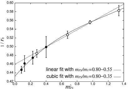
Figure 24: Chiral extrapolation of $r_{0}$. Open symbols are the results in our previous study Spectrum.Nf2.CP-PACS .

The results are seen in Fig. 24 and Table 9.

IV.4 Results at the physical point

The physical point is defined by empirical pion and $\rho$ meson masses, $M_{\pi}=0.1350$ GeV and $M_{\rho}=0.7711$ GeV. With our polynomial fit, the physical point $m_{\pi}$ for $m_{PS}$ is determined by solving the equation,

$$\frac{m_{\pi}}{A^{V}+B^{V}m_{\pi}^{2}+D^{V}m_{\pi}^{4}+F^{V}m_{\pi}^{6}}=\frac{M_{\pi}}{M_{\rho}}.$$ (38)

The $\rho$ meson mass at the physical point $m_{\rho}$ is obtained by Eq. (34) with $m_{PS}=m_{\pi}$, which determines the lattice spacing $a_{\rho}=0.2007(38)$ fm. The lattice spacing can also be determined from $r_{0}$ taking its phenomenological value $R_{0}=0.49$ fm. Using Eq. (37) instead of Eq. (34), we have

$$\frac{m_{\pi}}{A^{r_{0}}+B^{r_{0}}m_{\pi}^{2}+D^{r_{0}}m_{\pi}^{4}+F^{r_{0}}m_{\pi}^{6}}=M_{\pi}R_{0}.$$ (39)

Substitution of $m_{\pi}$ to Eq. (37) leads to $r_{0}$ at the physical point, yielding an alternative lattice spacing $a_{r_{0}}$, $a_{r_{0}}=0.2119(61)$ fm, which is consistent with $a_{\rho}$ within $2\sigma$.

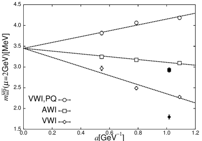
Figure 25: Comparison of degenerate up and down quark masses obtained by chiral extrapolations with polynomials. Open symbols show the results obtained in the previous calculation Spectrum.Nf2.CP-PACS and filled symbols are our new results. Lines are combined linear continuum extrapolations in the previous calculation.

We calculate $m_{ud}^{VWI}$ using $\kappa_{ud}$ defined by $m_{PS}(\kappa_{ud})=m_{\pi}$, and $m_{ud}^{AWI}$ by Eq. (33), and then convert to renormalized quark masses in the $\overline{\mbox{MS}}$ scheme at 2 GeV (see Sec. III.2). Table 10 presents a summary of the parameters at the physical point, obtained with polynomial extrapolations, together with comparisons with the quadratic fit in the previous work. The difference between old and new results is generally 4–8% except for the VWI quark mass for which a difference more than 20% is observed (see Fig. 25). The latter is caused by a shift of $\kappa_{c}$, with which even a small shift leads to an amplified change in the mean up and down quark mass.

V Chiral extrapolation based on ChPT

We first examine the one-loop formulae from continuum ChPT, which have already been tested in Spectrum.Nf2.JLQCD ; qq+q . We then attempt a fit based on WChPT including effects of $O(a^{2})$ chiral symmetry violation due to the Wilson term.

V.1 ChPT extrapolation

The one-loop formulae ChPT.Gasser ; PQChPT.Durr derived from ChPT in the continuum limit are

$$\frac{m_{PS}^{2}}{2B_{0}m_{quark}} = 1+\frac{1}{2}\frac{2B_{0}m_{quark}}{(4\pi f)^{2}}\log\frac{2B_{0}m_{quark}}{\Lambda_{3}^{2}}$$ (40)

$$f_{PS} = f\left(1-\frac{2B_{0}m_{quark}}{(4\pi f)^{2}}\log\frac{2B_{0}m_{quark}}{\Lambda_{4}^{2}}\right),$$ (41)

where $B_{0}$, $f$, $\Lambda_{3}$ and $\Lambda_{4}$ are parameters to be obtained by fits. The coefficient $1/2$ in front of the logarithm is a distinctive prediction of ChPT. Since several parameters are common in the two formulae, we fit $m_{PS}^{2}$ and $f_{PS}$ simultaneously. Correlations between $m_{PS}^{2}$ and $f_{PS}$ are neglected in the fits for simplicity. Thus, the $\chi^{2}/dof$ serves only as a guide to judge the relative quality of the fits. We estimate the errors by the jackknife method. We try both $m_{quark}^{AWI}$ and $m_{quark}^{VWI}$ (Cases 1 and 2 in what follows) for $m_{quark}$ that appears in these formulae. For $m_{quark}=m_{quark}^{VWI}$, we use $\kappa_{c}$ determined in Eq. (33) since $m_{quark}^{AWI}$ has no logarithmic singularities in ChPT. From the fits summarized in Table 11, we find:

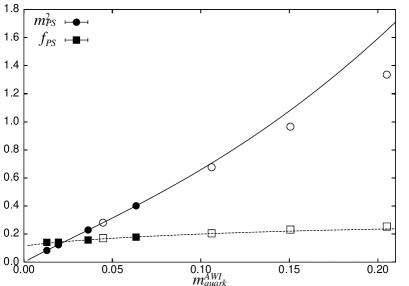
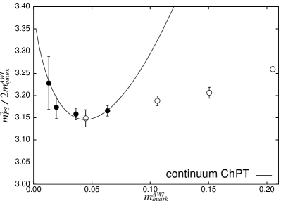
Figure 26: Test of simultaneous continuum ChPT fit to pseudoscalar meson mass and decay constant. In this plot, quark mass defined through the axial vector Ward identity is used. The right panel shows the ratio $m_{PS}^{2}/2m_{quark}^{AWI}$ to focus on the chiral logarithm behavior. Open symbols are the results obtained in our previous study Spectrum.Nf2.CP-PACS .

1. ($m_{quark}=m_{quark}^{AWI}$) : When we fit the data over the whole range $m_{PS}/m_{V}=0.80$–0.35, we are led to a large $\chi^{2}/dof\sim 70$. By restricting the fitting interval to $m_{PS}/m_{V}=0.60$–0.35 we obtain a reasonable fit with $\chi^{2}/dof=1.9$, which is plotted in Fig. 26. As one observes in the second panel of this figure, which shows $m_{PS}^{2}/2m_{quark}^{AWI}$ appearing in the left hand side of Eq.(40), the chiral logarithm may be visible only at $m_{PS}/m_{V}\,\hbox to0.0pt{\lower 3.5pt\hbox{$\mathchar 0\relax\sim$}\hss}\raise 1.0pt\hbox{$<$}\,0.40$.

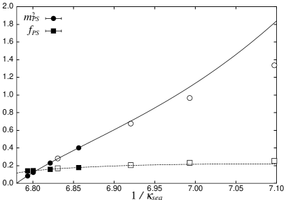
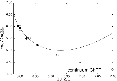
Figure 27: Test of simultaneous continuum ChPT fit with the quark mass defined through the vector Ward identity. Open symbols are the results obtained in our previous study Spectrum.Nf2.CP-PACS .

2. ($m_{quark}=m_{quark}^{VWI}$) : In contrast to Case 1, $m_{PS}^{2}/2m_{quark}^{VWI}$ increases toward the chiral limit in the whole mass range, which is seen in Fig. 27. Nevertheless, the situation is similar. A fit over the whole range $m_{PS}/m_{V}=0.80$–0.35 leads to $\chi^{2}/dof\sim 100$. To obtain an acceptable fit, we have to remove the data at large quark masses. The best fit obtained for the range $m_{PS}/m_{V}=0.60$–0.35 is shown in Fig. 27.

In neither case do we draw the clear evidence for the chiral logarithm for pseudoscalar mesons.

For the vector meson, we adopt the formula based on ChPT in the static limit ChPT.Jenkins .

$$m_{V}=A^{V}+B^{V}m_{PS}^{2}+C^{V}m_{PS}^{3}.$$ (42)

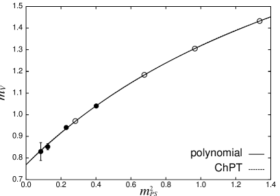
Figure 28: Chiral extrapolation of vector meson mass with a polynomial in Eq. (34) and a function motivated by ChPT in Eq. (42). Open symbols are the results obtained in our previous study Spectrum.Nf2.CP-PACS .

This cubic form describes our data well as shown in Fig. 28 (see Table 12 for numbers).

For octet and decuplet baryons we employ a similar cubic formula ChPT.Bernard

$$m_{oct,dec}=A^{oct,dec}+B^{oct,dec}m_{PS}^{2}+C^{oct,dec}m_{PS}^{3},$$ (43)

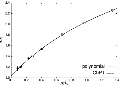
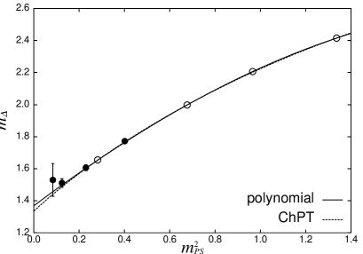
Figure 29: Chiral extrapolation of octet (left panel) and decuplet (right panel) baryon masses with polynomials in Eq. (36) and functions motivated by ChPT in Eq. (43). Open symbols are the results obtained in our previous study Spectrum.Nf2.CP-PACS .

which also reproduces our data well (Fig. 29 and Table 13).

In order to present predictions at the physical point, we carry out extrapolations using the data at $m_{PS}/m_{V}=0.60$–0.35. From Eq. (42) the physical point $m_{\pi}$ for $m_{PS}$ is given by

$$\frac{m_{\pi}}{A^{V}+B^{V}m_{\pi}^{2}+C^{V}m_{\pi}^{3}}=\frac{M_{\pi}}{M_{\rho}}.$$ (44)

The lattice spacing is determined to be $a_{\rho}^{ChPT}=0.192(10)$ fm. For the vector meson, a fit for the whole range $m_{PS}/m_{V}=0.80$–0.35 is acceptable, as seen in Table 12. We will use this fit in Sec. V.2 with $a_{\rho}^{ChPT}=0.2009(21)$ fm for this case.

The masses of non-strange baryons $N$ and $\Delta$ are determined by substituting $m_{\pi}$ to $m_{PS}$ in Eq. (43). The bare quark mass at the physical point $m_{ud}$ and the pion decay constant $f_{\pi}$ are obtained from Eqs. (40) and (41). Renormalized quark masses are calculated with $m_{ud}$ as in the case of polynomial extrapolations. These results are compiled in Table 14.

We observe 5–10% differences between the ChPT fits over $m_{PS}/m_{V}=0.60$–0.35 and the quadratic polynomial fits over $m_{PS}/m_{V}=0.80$–0.55 obtained in the previous work. The numbers are tabulated in Table 10. These differences are similar in magnitude to those we found with higher order polynomial extrapolations using the whole range $m_{PS}/m_{V}=0.80$–0.35. An exception is the VWI quark mass on which we shall make a further comment below.

V.2 WChPT extrapolation

V.2.1 WChPT without resummation

ChPT adapted to Wilson-type quark actions on the lattice (WChPT) has been addressed in Refs. WChPT.Sharpe ; WChPT.Rupak ; WChPT.Oliver ; WChPT.Sinya . An important point WChPT.Sinya is that $O(a^{2})$ chiral breaking terms in the chiral Lagrangian are essential to generate the parity-flavor breaking phase transition WChPT.Sharpe , which is necessary to explain the existence of massless pions for Wilson-type quark actions Aoki_phase.Sinya1 ; Aoki_phase.Sinya2 ; Aoki_phase.Sinya3 . Therefore, we must include the $O(a^{2})$ terms in the leading order. In this counting scheme, the one-loop formulae read WChPT.Sinya ,

$$m_{PS}^{2} = Am_{quark}^{VWI}\left(1+\omega_{1}^{PS}m_{quark}^{VWI}\log\left(\frac{Am_{quark}^{VWI}}{\Lambda_{3}^{2}}\right)+\omega_{0}\log\left(\frac{Am_{quark}^{VWI}}{\Lambda_{0}^{2}}\right)\right),$$ (45)

$$m_{quark}^{AWI} = m_{quark}^{VWI}\left(1+\omega_{1}^{AWI}m_{quark}^{VWI}\log\left(\frac{Am_{quark}^{VWI}}{\Lambda_{3,AWI}^{2}}\right)+\omega_{0}\log\left(\frac{Am_{quark}^{VWI}}{\Lambda_{0}^{2}}\right)\right),$$ (46)

$$f_{PS} = f\left(1-\omega_{1}^{f_{PS}}m_{quark}^{VWI}\log\left(\frac{Am_{quark}^{VWI}}{\Lambda_{4}^{2}}\right)\right).$$ (47)

Here $\kappa_{c}$ in $m_{quark}^{VWI}$, $A$, $f$, $\omega_{0}$, $\omega_{1}^{PS}$, $\omega_{1}^{AWI}$, $\omega_{1}^{f_{PS}}$, $\Lambda_{3}$, $\Lambda_{3,AWI}$, $\Lambda_{0}$ and $\Lambda_{4}$ are free parameters, and the overall factor of $m_{quark}^{AWI}$ is absorbed in $\omega_{0}$ and $\Lambda_{0}$. We note that $A$ consists of $O(a^{0})$ and $O(a^{1})$ parts, $\omega_{0}\sim O(a^{2})$, $\omega_{1}^{AWI}\sim O(a)$ and

$$\omega_{1}^{PS} = \frac{1}{2}\frac{(A+w_{1}^{\pi}a)}{(4\pi f_{0})^{2}},$$ (48)

$$\omega_{1}^{f_{PS}} = \frac{(A+w_{1}^{f_{\pi}}a)}{(4\pi f_{0})^{2}},$$ (49)

where $f_{0}$ is the pion decay constant in the continuum and chiral limit, which can be different from $f$ by $O(a)$. The constants $w_{1}^{\pi}$ and $w_{1}^{f_{\pi}}$ are $O(a^{0})$.

There are two features in these formulae worth emphasizing. First, the coefficients of $m_{quark}\log m_{quark}$ terms receive contributions of $O(a)$. This is in contrast to continuum ChPT, in which these coefficients take universal values. Second, there are terms of the form $a^{2}\log m_{quark}$ which are more singular than the $m_{quark}\log m_{quark}$ terms toward the chiral limit at a finite lattice spacing. Thus WChPT formulae predict the chiral behavior at finite lattice spacings that is different from what is expected from ChPT in the continuum limit.

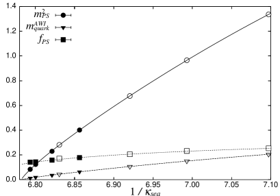
Figure 30: Test of the WChPT fit to pseudoscalar meson mass, AWI quark mass and decay constant. The right panel shows the ratio $m_{PS}^{2}/2m_{quark}^{AWI}$ to focus on the chiral logarithm behavior. Open symbols are the results obtained in our previous study Spectrum.Nf2.CP-PACS .

We fit $m_{PS}$ and $m_{quark}^{AWI}$ simultaneously, neglecting correlations between them. The errors are estimated by the jackknife method. We then fit $f_{PS}$ with $A$ and $\kappa_{c}$ fixed from Eqs. (45) and (46). We give the results in Fig. 30 and Tables 15 and 16. Fig. 30 demonstrates that the one-loop WChPT formulae explain our data over the whole range $m_{PS}/m_{V}=0.80$–0.35.

V.2.2 Resummed WChPT

While fits with Eqs. (45) and (46) work well for the whole range of quark mass we measured, extrapolation to the physical point is still problematic because the $\omega_{0}\log m_{quark}^{VWI}$ terms become larger than the leading terms in the chiral limit. A way out has been proposed in Ref. WChPT.Sinya in which leading singularities around the chiral limit is resummed. The resulting formulae read,

$$m_{PS}^{2} = Am_{quark}^{VWI}\left(-\log\left(\frac{Am_{quark}^{VWI}}{\Lambda_{0}^{2}}\right)\right)^{\omega_{0}}\left(1+\omega_{1}^{PS}m_{quark}^{VWI}\log\left(\frac{Am_{quark}^{VWI}}{\Lambda_{3}^{2}}\right)\right),$$ (50)

$$m_{quark}^{AWI} = m_{quark}^{VWI}\left(-\log\left(\frac{Am_{quark}^{VWI}}{\Lambda_{0}^{2}}\right)\right)^{\omega_{0}}\left(1+\omega_{1}^{AWI}m_{quark}^{VWI}\log\left(\frac{Am_{quark}^{VWI}}{\Lambda_{3,AWI}^{2}}\right)\right),$$ (51)

where the fitting parameters are $\kappa_{c}$ in $m_{quark}^{VWI}$, $A$, $\omega_{0}$, $\omega_{1}^{PS}$, $\omega_{1}^{AWI}$, $\Lambda_{3}$, $\Lambda_{3,AWI}$ and $\Lambda_{0}$. The minus sign in the resummed part is introduced to keep $-\log(Am_{quark}^{VWI}/\Lambda_{0}^{2})$ positive. We note that $f_{PS}$ is not affected by the resummation except for a shift of $\kappa_{c}$.

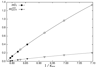
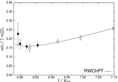
Figure 31: Test of the resummed WChPT fit to pseudoscalar meson mass and AWI quark mass. The right panel shows the ratio $m_{PS}^{2}/2m_{quark}^{AWI}$ to focus on the chiral logarithm behavior. Open symbols are the results obtained in our previous study Spectrum.Nf2.CP-PACS .

As with the case of WChPT without resummation, these resummed WChPT formulae describe our data for the whole range of $m_{PS}/m_{V}=0.80$–0.35. The results are seen in Fig. 31 and Tables 17 and 18.

The magnitude of the leading and the one-loop contributions is plotted in Fig. 32 as a function of $m_{quark}$. In contrast to WChPT without resummation, which is shown in the second panel of the figure, the one-loop contribution of resummed WChPT fit remains small in the the whole range of quark mass we explored, including the chiral limit. This confirms the convergence of the resummed WChPT formulae. Furthermore, the resulting parameters are comparable with phenomenological estimates; we obtain $\Lambda_{3}=0.15(15)$ [GeV] and $\Lambda_{4}=2.44(13)$ [GeV] as compared to $\Lambda_{3}=0.2$–2.0 [GeV] and $\Lambda_{4}=1.26(14)$ [GeV], respectively, from Ref. ChPT.Gasser ; Lambda_4.Colangelo . A more accurate examination requires extrapolation to the continuum limit, which is left for studies in the future.

In the present fit, the $m_{quark}\log m_{quark}$ terms are sizably suppressed due to $O(a)$ corrections for the pseudoscalar meson mass. In the combination $m_{PS}^{2}/2m_{quark}^{AWI}$, $(\omega_{1}^{PS}-\omega_{1}^{AWI})$ represents the strength of the chiral logarithm. The resummed WChPT fit gives $(\omega_{1}^{PS}-\omega_{1}^{AWI})=0.24(13)$, while in continuum ChPT we expect $\omega_{1}^{PS}=A/32\pi^{2}f_{0}^{2}=2.7$ and $\omega_{1}^{AWI}=0$, with the phenomenological value of $f_{0}=0.086$ GeV, ignoring $O(a)$ dependence in $A$. Namely, the coefficient of the logarithm is suppressed to about 10% of the ChPT value by $O(a)$ contributions in $m_{PS}^{2}$ and $m_{quark}^{AWI}$. It is important to repeat a similar analysis at a smaller lattice spacing to verify that the magnitude of the $m_{quark}\log m_{quark}$ coefficient converges toward the value predicted by ChPT.

V.2.3 Results at the physical point

Since WChPT formulae are not available for the vector meson, we adopt Eq. (42) to fix the physical point for $m_{\pi}$. A fit for the whole data in the range $m_{PS}/m_{V}=0.80$–0.35 yields $a_{\rho}^{ChPT}=0.2009(21)$ fm. Substituting $m_{\pi}$ to Eq. (50) and using $a_{\rho}^{ChPT}$, we obtain the VWI quark mass at the physical point $m_{ud}^{VWI}$. Eqs. (51) and (47) with $m_{ud}^{VWI}$ then yield $m_{ud}^{AWI}$ and $f_{\pi}$ respectively (Table 19).

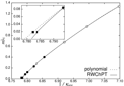
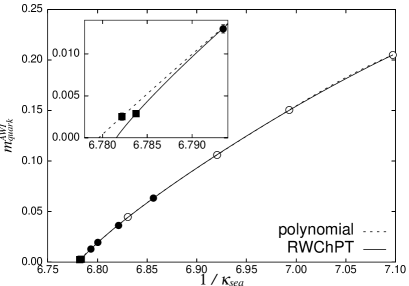
Figure 33: Comparisons of the polynomial and the resummed WChPT fits to pseudoscalar meson mass and AWI quark mass determined at $m_{PS}/m_{V}=0.80$–0.35. Circles show the lattice data and the square is the extrapolated result at the physical point. Open symbols are the results obtained in our previous study Spectrum.Nf2.CP-PACS .

Let us compare the resummed WChPT results with those of the quadratic polynomial obtained with the original data over the range $m_{PS}/m_{V}=0.80$–0.55 (Table 10) and the fits using ChPT formula in the continuum limit for $m_{PS}/m_{V}=0.60$–0.35 (Table 14). The lattice spacing, the AWI quark mass, and the pion decay constant take similar values among higher order polynomials, ChPT and resummed WChPT formulae. An exception is the VWI quark mass which significantly depends on the functional forms for the chiral extrapolation. (see Fig. 33). Our final values for the light quark mass at $a=0.2$ fm are:

$$m_{ud}^{VWI,\overline{\rm MS}}(\mu=2~{}\mbox{GeV}) = \left\{\begin{array}[]{l}1.314(99)\mbox{~{}[MeV]}\hskip 14.22636pt\mbox{ (resummed WChPT) }\\ 1.796(51)\mbox{~{}[MeV]}\hskip 14.22636pt\mbox{ (polynomial) }\end{array}\right.$$ (54)

$$m_{ud}^{AWI,\overline{\rm MS}}(\mu=2~{}\mbox{GeV}) = \left\{\begin{array}[]{l}2.902(36)\mbox{~{}[MeV]}\hskip 14.22636pt\mbox{ (resummed WChPT) }\\ 2.927(53)\mbox{~{}[MeV]}\hskip 14.22636pt\mbox{ (polynomial) }\end{array}\right.$$ (57)

The sensitivity of the VWI quark mass on the functional form of chiral extrapolation is due to closeness of $\kappa_{ud}$ to the critical value $\kappa_{c}$. A small variation of $\kappa_{c}$ is easily amplified in the up and down quark mass which is determined by the difference $1/\kappa_{ud}-1/\kappa_{c}$.

V.2.4 Chiral extrapolation from large quark masses

Finally, we test if WChPT explains the deviations of our new data at small quark masses from the quadratic extrapolation of the data at $m_{PS}/m_{V}=0.80$–0.55. A motivation of this test is the rapid increase of the computational time to simulate QCD toward small sea quark masses on fine lattices. If WChPT correctly predicts the small quark mass behavior from heavy sea quark mass simulations for $m_{PS}/m_{V}\geq 0.5$, it will be a great help for our studies.

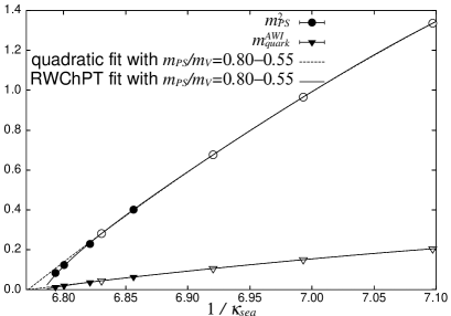
Figure 34: Comparison of quadratic and resummed WChPT fits to pseudoscalar meson masses and AWI quark masses determined from the previous data of $m_{PS}/m_{V}=0.80$–0.55 Spectrum.Nf2.CP-PACS (open symbols) with the new small sea quark mass data (filled symbols). The right panel is an enlargement around the chiral limit.

We apply the resummed WChPT formulae to the large quark mass data set at $\beta=1.80$. Since the number of data points at $m_{PS}/m_{V}\geq 0.5$ is small for a stable fitting, we introduce a restriction: $\Lambda_{3}=\Lambda_{3,AWI}$. Fig. 34 (see Table 19 for numerical values) compares the fit from the large quark mass data set and that using the data for the entire mass range. The resummed WChPT fit using the large quark mass data set alone describes the small sea quark mass data very well. This contrasts to the polynomial extrapolation. Our observation suggests that WChPT may provide a valuable tool to carry out an accurate chiral extrapolation using simulations with not too small quark masses.

Encouraged by this, we apply the resummed WChPT to the two additional data sets at $m_{PS}/m_{V}=0.80$–0.55 obtained at smaller lattice spacings at $\beta=1.95$ and 2.1 ($a=0.16$ and 0.11 fm) in the previous work. A simultaneous linear continuum extrapolation using $m_{ud}^{VWI,\overline{\rm MS}}$ and $m_{ud}^{AWI,\overline{\rm MS}}$, combined with the results for $\beta=1.8$, leads to

$$m_{ud}^{\overline{\rm MS}}(\mu=2~{}\mbox{GeV})=3.06(18)\mbox{~{}[MeV]}\hskip 14.22636pt\mbox{ (resummed WChPT fit) }$$ (58)

where the error is statistical only. When we use our whole data of $m_{PS}/m_{V}=0.80$–0.35 at $\beta=1.80$, we obtain

$$m_{ud}^{\overline{\rm MS}}(\mu=2~{}\mbox{GeV})=3.11(17)\mbox{~{}[MeV]}\hskip 14.22636pt\mbox{ (resummed WChPT fit with our whole data) }$$ (59)

This is compared to our previous result using the quadratic extrapolation:

$$m_{ud}^{\overline{\rm MS}}(\mu=2~{}\mbox{GeV})=3.45(10)\mbox{~{}[MeV]}\hskip 14.22636pt\mbox{ (quadratic fit) }$$ (60)

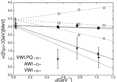
Figure 35: Continuum extrapolations of degenerate up and down quark mass obtained by chiral extrapolations with polynomials Spectrum.Nf2.CP-PACS (open symbols) and the resummed WChPT formulae (filled symbols). The star at $a\simeq 1\,{\rm GeV}^{-1}$ ($\beta=1.8$) represents the results obtained by the resummed WChPT formulae with data at $m_{PS}/m_{V}=0.80$–0.35. The others are the results with $m_{PS}/m_{V}=0.80$–0.55. The dashed lines are the combined linear fit to the quadratic chiral fit results and the dashed-dot lines are the ones to the resummed WChPT fit results, both with $m_{PS}/m_{V}=0.80$–0.55. The solid lines are the combined linear fits to the resummed WChPT chiral fit results with our whole data of $m_{PS}/m_{V}=0.80$–0.35 at $\beta=1.8$ and $m_{PS}/m_{V}=0.80$–0.55 at $\beta=1.95$ and 2.1.

The resummed WChPT results in a 10% decrease in the mean up and down quark mass. This is demonstrated in Fig. 35.

VI Conclusions

In this paper, we have pushed our previous study of two-flavor QCD down to a sea quark mass as small as $m_{PS}/m_{V}=0.35$, using the RG-improved gauge action and the clover-improved Wilson quark action. We have found that our new data at $m_{PS}/m_{V}=0.60$–0.35 show clear deviations from the prediction of the previous chiral extrapolations based on quadratic polynomials, which implies that higher order terms were needed to describe the behavior at a small sea quark mass. On the other hand, our current data do not show the clear quark mass dependence expected from ChPT in the continuum: the chiral logarithm may appear only below $m_{PS}/m_{V}\sim 0.4$. This result contrasts with that of the qq+q collaboration qq+q based on unimproved plaquette glue and Wilson quark actions, but is not dissimilar to that of UKQCD Spectrum.Nf2.UKQCD_light .

We have provisionally ascribed the major reason for the failure of continuum ChPT to explicit chiral symmetry breaking of the Wilson term, which is significant on our lattice of $a=0.2$ fm. We have then made a test of WChPT in which the effect of the Wilson term is accommodated, and found the resummed one-loop WChPT formulae that take account of the effects up to $O(a^{2})$ describe well our entire data. Convergence tests indicate that resummed WChPT gives well-controlled chiral extrapolations. The use of WChPT generally leads to modifications of various physical observables at the physical point by about 10%, compared with those obtained in the quadratic extrapolation at this lattice spacing. A much larger modification, however, is seen with the light quark mass defined through vector Ward identity: the WChPT extrapolation decreases it by 30%.

We note in particular that the resummed WChPT extrapolation from our previous data at $m_{PS}/m_{V}=0.80$–0.55 predicts correctly the new data at $m_{PS}/m_{V}=0.60$–0.35. Encouraged by this fact, we attempted a continuum extrapolation of the light quark mass using the resummed WChPT fits to the previous data at $m_{PS}/m_{V}=0.80$–0.55 but on finer lattices with $a=0.16$ and 0.11 fm. We find in the continuum limit, $m_{ud}^{\overline{\rm MS}}(\mu=2~{}\mbox{GeV})=3.11(17)$ [MeV], which is smaller than the previously reported result by approximately 10%. Our work suggests that WChPT provides us with a valuable theoretical framework for chiral extrapolations.

Appendix A Hadron masses

Measured hadron masses are summarized in Tables 20 – 27. Our choice of the fitting range and resulting value of $\chi^{2}/{dof}$ are also given in these tables.

Table 1: Run parameters of the present simulation. The step size $dt$ is given by the inverse of the number of the molecular dynamics steps (#MD), and hence not listed. We denote the tolerance parameter in the stopping condition for the quark matrix inversion in calculations of the force by $\Delta_{force}$ and the average number of iterations by $N_{inv}$. Number of node (PE’s) of VPP5000/80 used for the present calculation, and the CPU time required per trajectory in units of hour are also given. The number of trajectory is denoted by $N_{traj}$.

$12^{3}\times 24$	on 4PE		on 4PE		on 4PE		on 8PE
$\kappa_{sea}$	0.14585		0.14660		0.14705		0.14720
#MD	200		333	400	800	1000	1250	1600
Accept.	0.76		0.72	0.84	0.82	0.90	0.87	0.91
$N_{traj}$	4000		1750	2250	680	3320	100	1300
$\Delta_{force}$	$10^{-10}$		$10^{-11}$		$10^{-11}$		$10^{-12}$
$N_{inv}$	87		147		232		318
Hour/traj.	0.23		0.56	0.69	2.0	2.6	2.2	3.2
$m_{PS}/m_{V}$	0.609(2)		0.509(5)		0.413(8)		0.349(19)
$16^{3}\times 24$	on 4PE		on 8PE
$\kappa_{sea}$	0.14585		0.14660		0.14705		0.14720
#MD	200	250	333	500	–		–
Accept.	0.61	0.71	0.79	0.80	–		–
$N_{traj}$	800	1200	325	1675	–		–
$\Delta_{force}$	$10^{-10}$		$10^{-11}$		–		–
$N_{inv}$	92		158		–		–
Hour/traj.	0.50	0.61	0.69	1.03	–		–
$m_{PS}/m_{V}$	0.604(3)		0.509(4)		–		–

Table 2: String tension $\sigma$ and Sommer scale $r_{0}$ at simulated sea quark masses. The first error is statistical. The second and third ones are the systematic errors due to the choice of $t_{min}$ and $r_{min}$.

$12^{3}\times 24$
$\kappa_{sea}$	$t_{min}$	$r_{min}$	$\sigma$	$r_{0}$
0.14585	2	$\sqrt{2}$	0.322(6)($-42$)($+91$)	2.004(8)($+58$)($+77$)
0.14660	2	$\sqrt{2}$	0.289(5)($-8$)($+64$)	2.107(8)($+37$)($+54$)
0.14705	2	$\sqrt{2}$	0.278(5)($-38$)($+34$)	2.167(9)($+80$)($+25$)
0.14720	2	$\sqrt{2}$	0.255(8)($-10$)($+42$)	2.237(17)($+10$)($+34$)
$16^{3}\times 24$
$\kappa_{sea}$	$t_{min}$	$r_{min}$	$\sigma$	$r_{0}$
0.14585	2	$\sqrt{2}$	0.313(11)($-10$)($+90$)	2.011(10)($+17$)($+72$)
0.14660	2	$\sqrt{2}$	0.270(6)($+7$)($+66$)	2.131(11)($+20$)($+39$)

Table 3: Autocorrelation time for plaquette ($\tau^{cum}_{plaq}$), pseudoscalar meson propagator at $N_{t}/4$ ($\tau^{cum}_{PS}$) and Wilson loop with $(r,t)=(2,2)$ ($\tau^{cum}_{W}$). All values are in units of HMC trajectory.

$12^{3}\times 24$
$\kappa_{sea}$	0.14585	0.14660	0.14705	0.14720
$\tau^{cum}_{plaq}$	7.6(1.8)	11.7(2.3)	9.5(2.1)	8.9(3.2)
$\tau^{cum}_{PS}$	7.9(1.6)	7.2(1.5)	5.3(1.2)	3.0(1.0)
$\tau^{cum}_{W}$	8.1(1.9)	12.6(2.9)	11.3(2.2)	13.0(4.4)
$16^{3}\times 24$
$\kappa_{sea}$	0.14585	0.14660	0.14705	0.14720
$\tau^{cum}_{plaq}$	14.1(3.9)	8.8(2.1)	–	–
$\tau^{cum}_{PS}$	10.3(2.8)	4.9(1.6)	–	–
$\tau^{cum}_{W}$	14.1(3.8)	10.1(4.3)	–	–

Table 4: Parameters of independent polynomial chiral fits to AWI quark masses and pseudoscalar meson masses as a function of the VWI quark mass.

$m_{PS}/m_{V}$	$\kappa_{c}$	$B^{AWI}$	$C^{AWI}$	$D^{AWI}$	$E^{AWI}$	$\chi^{2}/dof$	$Q$
0.80–0.35	0.147502(14)	1.961(60)	$-10.5(1.9)$	71(20)	$-201(67)$	4.38/3	0.22
$m_{PS}/m_{V}$	$\kappa_{c}$	$B^{PS}$	$C^{PS}$	$D^{PS}$	$E^{PS}$	$\chi^{2}/dof$	$Q$
0.80–0.35	0.147514(15)	12.05(33)	$-55.7(9.0)$	359(89)	$-966(281)$	4.17/3	0.24

Table 5: Parameters of simultaneous polynomial chiral fits to AWI quark masses and pseudoscalar meson masses as a function of the VWI quark mass. The first error is statistical and the second is a systematic one due to the higher order term for the chiral extrapolation.

$m_{PS}/m_{V}$	$\kappa_{c}$	$B^{AWI}$	$C^{AWI}$	$D^{AWI}$	$E^{AWI}$	$\chi^{2}/dof$
0.80–0.35	0.147508(14)(+7)	$1.938(54)(-60)$	$-9.8(1.7)(+3.3)$	$65(18)(-67)$	$-181(60)(+541)$	8.89/7
		$B^{PS}$	$C^{PS}$	$D^{PS}$	$E^{PS}$	$Q$
		$12.18(31)(-20)$	$-58.9(8.6)(+7.9)$	$389(85)(-126)$	$-1053(269)(+880)$	0.26

Table 6: Parameters of polynomial chiral fits to vector meson mass. The first error is statistical and the second is a systematic one due to the higher order term for the chiral extrapolation.

$m_{PS}/m_{V}$	$A^{V}$	$B^{V}$	$D^{V}$	$F^{V}$	$\chi^{2}/{dof}$	$Q$
0.80–0.35	$0.770(15)(-6)$	$0.790(72)(+47)$	$-0.304(97)(-116)$	$0.063(39)(+113)$	1.10/4	0.89

Table 7: Parameters of polynomial chiral fits to pseudoscalar and vector meson decay constants.

$m_{PS}/m_{V}$	$A^{f_{PS}}$	$B^{f_{PS}}$	$D^{f_{PS}}$	$F^{f_{PS}}$	$\chi^{2}/{dof}$	$Q$
0.80–0.35	$0.1239(26)(-83)$	$0.165(17)(+86)$	$-0.076(27)(-264)$	$0.018(12)(+296)$	17.2/4	0.0018
$m_{PS}/m_{V}$	$A^{f_{V}}$	$B^{f_{V}}$	$D^{f_{V}}$	$F^{f_{V}}$	$\chi^{2}/{dof}$	$Q$
0.80–0.35	$0.228(12)(-15)$	$0.265(59)(+127)$	$-0.156(85)(-336)$	$0.039(35)(+340)$	2.31/4	0.68

Table 8: Parameters of polynomial chiral fits to octet and decuplet baryon masses.

$m_{PS}/m_{V}$	$A^{oct}$	$B^{oct}$	$D^{oct}$	$F^{oct}$	$\chi^{2}/{dof}$	$Q$
0.80–0.35	$1.051(23)(+21)$	$1.41(12)(-19)$	$-0.51(18)(+56)$	$0.097(78)(-591)$	4.96/4	0.29
$m_{PS}/m_{V}$	$A^{dec}$	$B^{dec}$	$D^{dec}$	$F^{dec}$	$\chi^{2}/{dof}$	$Q$
0.80–0.35	$1.381(37)(+8)$	$1.03(19)(-7)$	$-0.17(29)(+18)$	$-0.022(126)(-186)$	0.75/4	0.95

Table 9: Parameters of polynomial chiral extrapolation of $r_{0}$.

$m_{PS}/m_{V}$	$A_{r_{0}}$	$B_{r_{0}}$	$D_{r_{0}}$	$F_{r_{0}}$	$\chi^{2}/{dof}$	$Q$
0.80–0.35	$0.432(12)(-7)$	$0.207(89)(+99)$	$-0.11(14)(-32)$	$0.032(64)(+364)$	0.37/4	0.99

Table 10: Results of physical quantities obtained by polynomial chiral fits using data at $m_{PS}/m_{V}=0.80$–0.35. The results of the previous quadratic fits at $m_{PS}/m_{V}=0.80$–0.55 Spectrum.Nf2.CP-PACS are also shown. The first error is statistical and the second is a systematic one due to the higher order term for the chiral extrapolation. Only statistical errors are given for the previous results.

	Quartic fit (this study)	Quadratic fit Spectrum.Nf2.CP-PACS	Difference
fit range in $m_{PS}/m_{V}$	0.80–0.35	0.80–0.55
$a_{\rho}$[fm]	$0.2007(38)(-14)$	0.2150(22)	$-7\%(6.5\sigma)$
$\kappa_{ud}$	$0.147440(13)(+7)$	0.147540(16)	$-0.1\%(6.3\sigma)$
$m_{ud}^{VWI,\overline{\rm MS}}(\mu=2~{}\mbox{GeV})$[MeV]	$1.796(51)(+18)$	2.277(27)	$-21\%(18\sigma)$
$m_{ud}^{AWI,\overline{\rm MS}}(\mu=2~{}\mbox{GeV})$[MeV]	$2.927(53)(-55)$	3.094(35)	$-6\%(4.8\sigma)$
$f_{\pi}$[GeV]	$0.1248(31)(-59)$	0.1288(33)	$-3\%(1.2\sigma)$
$f_{\rho}$[GeV]	$0.2294(74)(-111)$	0.2389(47)	$-4\%(2.0\sigma)$
$m_{N}$[GeV]	$1.060(27)(+24)$	1.016(16)	$+4\%(2.8\sigma)$
$m_{\Delta}$[GeV]	$1.377(39)(+16)$	1.270(23)	$+8\%(4.7\sigma)$

Table 11: Chiral extrapolation of pseudoscalar meson masses and decay constants based on the continuum ChPT formulae at one-loop with $m_{quark}=m_{quark}^{AWI}$ and $m_{quark}=m_{quark}^{VWI}$. $\kappa_{c}$ has been determined with $m_{quark}^{AWI}$. The value of $\kappa_{c}$ is shown in Table 4.

$m_{PS}/m_{V}$	$B_{0}^{AWI}$	$f^{AWI}$	$\Lambda_{3}^{AWI}$	$\Lambda_{4}^{AWI}$	$\chi^{2}/dof$	$Q$
0.80–0.35	3.838(15)	0.12162(47)	1.553(10)	2.633(15)	849/12	$10^{-174}$
0.60–0.35	3.398(52)	0.1130(20)	0.902(71)	2.591(98)	11.2/6	0.083
$m_{PS}/m_{V}$	$B_{0}^{VWI}$	$f^{VWI}$	$\Lambda_{3}^{VWI}$	$\Lambda_{4}^{VWI}$	$\chi^{2}/dof$	$Q$
0.80–0.35	6.886(22)	0.13225(35)	2.4018(85)	2.463(11)	1417/12	$10^{-296}$
0.60–0.35	6.582(87)	0.1145(18)	1.645(83)	2.262(72)	17.5/6	0.0076

Table 12: Parameters of chiral fits to vector meson mass based on continuum ChPT.

$m_{PS}/m_{V}$	$A^{V}$	$B^{V}$	$C^{V}$	$\chi^{2}/{dof}$	$Q$
0.80–0.35	0.7692(86)	0.897(32)	$-0.346(23)$	1.39/5	0.93
0.60–0.35	0.731(45)	1.31(49)	$-0.85(60)$	0.33/2	0.85

Table 13: Parameters of chiral fits to octet and decuplet baryon masses based on continuum ChPT.

$m_{PS}/m_{V}$	$A^{oct}$	$B^{oct}$	$C^{oct}$	$\chi^{2}/{dof}$	$Q$
0.80–0.35	1.043(14)	1.641(68)	$-0.632(51)$	5.13/5	0.40
0.60–0.35	1.011(52)	2.08(59)	$-1.23(74)$	2.23/2	0.33
$m_{PS}/m_{V}$	$A^{dec}$	$B^{dec}$	$C^{dec}$	$\chi^{2}/{dof}$	$Q$
0.80–0.35	1.351(20)	1.353(88)	$-0.481(66)$	1.24/5	0.94
0.60–0.35	1.428(86)	0.52(93)	0.53(1.15)	0.23/2	0.89

Table 14: Results of physical quantities obtained by continuum one-loop ChPT chiral fits using data at $m_{PS}/m_{V}=0.60$–0.35. For the $m_{quark}=m_{quark}^{VWI}$ case, $\kappa_{c}$ has been fixed to the value determined from the quartic fit to $m_{quark}^{AWI}$ shown in Table 4. The errors are statistical.

	continuum ChPT $\left(m_{quark}=m_{quark}^{AWI}\right)$	continuum ChPT $\left(m_{quark}=m_{quark}^{VWI}\right)$
$a_{\rho}$[fm]	0.192(10)
$\kappa_{ud}$	0.147445(14)	0.1474431(65)
$m_{ud}^{VWI,\overline{\rm MS}}(\mu=2~{}\mbox{GeV})$[MeV]	1.609(89)	1.625(81)
$m_{ud}^{AWI,\overline{\rm MS}}(\mu=2~{}\mbox{GeV})$[MeV]	2.66(13)	2.68(13)
$f_{\pi}$[GeV]	0.1219(64)	0.1231(65)
$m_{N}$[GeV]	1.074(69)
$m_{\Delta}$[GeV]	1.47(11)

Table 15: Parameters of chiral fits to pseudoscalar meson and AWI quark masses based on WChPT.

$m_{PS}/m_{V}$	$\kappa_{c}$	$A$	$\omega_{0}$	$\omega_{1}^{PS}$	$\omega_{1}^{AWI}$	$\Lambda_{0}$	$\Lambda_{3}$	$\Lambda_{3}^{AWI}$	$\chi^{2}/{dof}$	$Q$
0.80–0.35	0.147445(27)	6.312(44)	$-0.40(13)$	$-2.0(1.4)$	$-2.0(1.4)$	0.91(35)	1.95(15)	1.77(23)	11.9/8	0.16

Table 16: Parameters of chiral fits to pseudoscalar meson decay constants based on WChPT. $\kappa_{c}$ and $A$ has been fixed to the values in Table 15.

$m_{PS}/m_{V}$	$f$	$\omega_{1}^{f_{PS}}$	$\Lambda_{4}$	$\chi^{2}/{dof}$	$Q$
0.80–0.35	0.1233(17)	3.73(30)	2.44(13)	18.1/5	0.0028

Table 17: Parameters of chiral fits to pseudoscalar meson and AWI quark masses based on the resummed WChPT.

$m_{PS}/m_{V}$	$\kappa_{c}$	$A$	$\omega_{0}$	$\omega_{1}^{PS}$	$\omega_{1}^{AWI}$	$\Lambda_{0}$	$\Lambda_{3}$	$\Lambda_{3}^{AWI}$	$\chi^{2}/{dof}$	$Q$
0.80–0.35	0.147459(20)	6.354(59)	0.542(46)	0.65(51)	0.42(49)	0.397(56)	0.15(15)	0.07(16)	11.0/8	0.20

Table 18: Parameters of chiral fits to pseudoscalar meson decay constants based on the resummed WChPT. $\kappa_{c}$ and $A$ has been fixed to the values in Table 17.

$m_{PS}/m_{V}$	$f$	$\omega_{1}^{f_{PS}}$	$\Lambda_{4}$	$\chi^{2}/{dof}$	$Q$
0.80–0.35	0.1227(17)	3.78(30)	2.44(13)	18.2/5	0.0028

Table 19: Results of physical quantities obtained by the resummed WChPT fits using data at $m_{PS}/m_{V}=0.80$–0.35. The results are compared with the results of the resummed WChPT fits using our previous data at $m_{PS}/m_{V}=0.80$–0.55.

	RWChPT	RWChPT	Difference
fit range in $m_{PS}/m_{V}$	0.80–0.35	0.80–0.55
$a_{\rho}$[fm]	0.2009(21)	0.2022(38)	$-1\%(0.3\sigma)$
$\kappa_{ud}$	0.147409(16)	0.14736(22)	$+0.03\%(0.2\sigma)$
$m_{ud}^{VWI,\overline{\rm MS}}(\mu=2~{}\mbox{GeV})$[MeV]	1.314(99)	1.10(64)	$+19\%(0.3\sigma)$
$m_{ud}^{AWI,\overline{\rm MS}}(\mu=2~{}\mbox{GeV})$[MeV]	2.902(36)	2.945(60)	$-1\%(0.7\sigma)$
$f_{\pi}$[GeV]	0.1238(21)	0.1368(43)	$-10\%(3.0\sigma)$

Table 20: Meson masses and bare AWI quark masses on $12^{3}\times 24$ lattice.

$\kappa_{sea}$	$m_{PS}$	[$t_{min},t_{max}$]	$\chi^{2}/dof$	$m_{V}$	[$t_{min},t_{max}$]	$\chi^{2}/dof$	$m_{quark}^{AWI}$
0.14585	0.6336(14)	[6,12]	0.76(84)	1.0405(38)	[6,12]	0.40(51)	0.06340(34)
0.14660	0.4789(23)	[6,12]	1.60(1.19)	0.9410(81)	[6,12]	2.36(1.02)	0.03632(39)
0.14705	0.3520(29)	[6,12]	0.60(77)	0.8526(148)	[6,12]	0.67(81)	0.01952(30)
0.14720	0.2893(61)	[6,12]	0.50(93)	0.8300(413)	[6,12]	0.95(92)	0.01296(49)

Table 21: Decay constants on $12^{3}\times 24$ lattice. Here for the renormalization factor we employ $\kappa_{c}$ determined from a simultaneous fit to $m_{PS}^{2}$ and $m_{quark}^{AWI}$ in Table 5.

$\kappa_{sea}$	$f_{PS}$	[$t_{min},t_{max}$]	$f_{V}$	[$t_{min},t_{max}$]
0.14585	0.1785(14)	[6,12]	0.3118(33)	[6,12]
0.14660	0.15784(87)	[6,12]	0.2874(57)	[6,12]
0.14705	0.1413(14)	[6,12]	0.2496(97)	[6,12]
0.14720	0.1412(41)	[6,12]	0.2422(239)	[6,12]

Table 22: Baryon masses on $12^{3}\times 24$ lattice.

$\kappa_{sea}$	$m_{N}$	[$t_{min},t_{max}$]	$\chi^{2}/dof$	$m_{\Delta}$	[$t_{min},t_{max}$]	$\chi^{2}/dof$
0.14585	1.5357(69)	[5,12]	0.65(76)	1.7722(97)	[5,12]	0.74(83)
0.14660	1.3619(92)	[5,12]	0.85(66)	1.6061(183)	[5,12]	1.45(97)
0.14705	1.2054(165)	[5,12]	0.69(96)	1.5110(268)	[5,12]	1.28(81)
0.14720	1.1791(417)	[5,12]	0.99(62)	1.5300(1020)	[5,12]	0.62(1.23)

Table 23: Plaquette and rectangular loops on $12^{3}\times 24$ lattice.

$\kappa_{sea}$	$\left\langle W^{1\times 1}\right\rangle$	$\left\langle W^{1\times 2}\right\rangle$
0.14585	0.504529(56)	0.249916(70)
0.14660	0.508445(69)	0.254866(88)
0.14705	0.511202(68)	0.258350(86)
0.14720	0.512632(144)	0.260157(186)

Table 24: Meson and bare AWI quark masses on $16^{3}\times 24$ lattice.

$\kappa_{sea}$	$m_{PS}$	[$t_{min},t_{max}$]	$\chi^{2}/dof$	$m_{V}$	[$t_{min},t_{max}$]	$\chi^{2}/dof$	$m_{quark}^{AWI}$
0.14585	0.6333(19)	[6,12]	0.72(52)	1.0488(43)	[6,12]	0.82(76)	0.06378(47)
0.14660	0.4781(16)	[6,12]	3.55(2.04)	0.9403(70)	[6,12]	1.41(93)	0.03642(40)

Table 25: Decay constants on $16^{3}\times 24$ lattice. Here for the renormalization factor we employ $\kappa_{c}$ determined from a simultaneous fit to $m_{PS}^{2}$ and $m_{quark}^{AWI}$ in Table 5.

$\kappa_{sea}$	$f_{PS}$	[$t_{min},t_{max}$]	$f_{V}$	[$t_{min},t_{max}$]
0.14585	0.1804(23)	[6,12]	0.3151(45)	[6,12]
0.14660	0.1592(16)	[6,12]	0.2913(48)	[6,12]

Table 26: Baryon masses on $16^{3}\times 24$ lattice.

$\kappa_{sea}$	$m_{N}$	[$t_{min},t_{max}$]	$\chi^{2}/dof$	$m_{\Delta}$	[$t_{min},t_{max}$]	$\chi^{2}/dof$
0.14585	1.5567(91)	[5,12]	1.97(92)	1.7804(113)	[5,12]	0.64(54)
0.14660	1.3257(118)	[5,12]	1.58(91)	1.5899(124)	[5,12]	0.96(77)

Table 27: Plaquette and rectangular loops on $16^{3}\times 24$ lattice.

$\kappa_{sea}$	$\left\langle W^{1\times 1}\right\rangle$	$\left\langle W^{1\times 2}\right\rangle$
0.14585	0.504482(75)	0.249850(90)
0.14660	0.508338(61)	0.254739(76)

Figure 1: Comparison of convergence with various algorithms for inversions of the quark matrix at $\kappa_{sea}=0.14585$ ($m_{PS}/m_{V}=0.60$) and $\kappa_{valence}=0.14850$ ($m_{PS}/m_{V}=0.27$) on $12^{3}\times 24$ lattice. Conventional BiCGStab corresponds to $L=1$. We define an iteration $N_{iter}$ as a dimension of the Krylov subspace to which approximate solutions belong BiCGStab_L.Sleijpen . The number of matrix-vector products to obtain an approximate solution is $2\times N_{iter}$.

Figure 7: Effective potential energies $V_{eff}(r=N_{s}/4,t)$ at $\kappa_{sea}=0.14705$ ($m_{PS}/m_{V}=0.40$) on $12^{3}\times 24$ lattice.

Figure 9: Autocorrelation function of plaquette at $\kappa_{sea}=0.14705$ ($m_{PS}/m_{V}=0.40$) on $12^{3}\times 24$ lattice.

Figure 12: Volume dependence of pseudoscalar (left panel) and vector meson masses (right panel) at $\kappa_{sea}=0.14585$ ($m_{PS}/m_{V}=0.60$) and $\kappa_{sea}=0.14660$ ($m_{PS}/m_{V}=0.50$).

Figure 13: Volume dependence of AWI quark masses at $\kappa_{sea}=0.14585$ ($m_{PS}/m_{V}=0.60$) and $\kappa_{sea}=0.14660$ ($m_{PS}/m_{V}=0.50$).

Figure 15: Volume dependence of Sommer scales at $\kappa_{sea}=0.14585$ ($m_{PS}/m_{V}=0.60$) and $\kappa_{sea}=0.14660$ ($m_{PS}/m_{V}=0.50$).

Figure 32: Ratio of the next-to-leading order term to the leading one for $m_{PS}^{2}$ with the resummed WChPT formulae (left panel) and with WChPT formulae without resummation (right panel) as a function of $m_{quark}^{VWI}$.

References

(1)
For a review, see
S. Aoki,
Nucl. Phys. B (Proc. Suppl.) 94, 3 (2001);
D. Toussaint,
Nucl. Phys. B (Proc. Suppl.) 106, 111 (2002);
T. Kaneko,
Nucl. Phys. B (Proc. Suppl.) 106, 133 (2002).
(2)
S.Aoki et al. (CP-PACS Collaboration),
Phys. Rev. Lett. 84, 238 (2000);
Phys. Rev. D 67, 034503 (2003).
(3)
A. Ali Khan et al. (CP-PACS Collaboration),
Phys. Rev. Lett. 85, 4674 (2000) [E: 90, 029902 (2003)];
Phys. Rev. D 65, 054505 (2002) [E: D 67, 059901 (2003)].
(4)
C. Bernard et al. (MILC Collaboration),
Nucl. Phys. B (Proc. Suppl.) 73, 198 (1999);
ibid.60A, 297 (1998) and
references therein.
(5)
N. Eicker et al. (SESAM Collaboration),
Phys. Rev. D 59, 014509 (1999).
(6)
T. Lippert, et al. (TL Collaboration),
Nucl. Phys. B (Proc. Suppl.) 60A, 311 (1998).
(7)
N. Eicker, Th. Lippert, B. Orth and K. Schilling
(SESAM-TL Collaboration),
Nucl. Phys. B (Proc. Suppl.) 106, 209 (2002).
(8)
C.R. Allton et al. (UKQCD Collaboration),
Phys. Rev. D 60, 034507 (1999).
(9)
C.R. Allton et al. (UKQCD Collaboration),
Phys. Rev. D 65, 054502 (2002).
(10)
H. Stüben, (QCDSF-UKQCD Collaboration),
Nucl. Phys. B (Proc. Suppl.) 94, 273 (2001).
(11)
S. Aoki et al. (JLQCD Collaboration),
Phys. Rev. D 68, 054502 (2003).
(12)
J. Gasser and H. Leutwyler,
Ann. Phys. 158, 142 (1984);
Nucl. Phys. B 250, 465;517;539 (1985).
(13)
S. R. Sharpe and N. Shoresh,
Phys. Rev. D 62, 094503 (2000).
(14)
S. Durr,
Eur. Phys. J. C 29, 383 (2003).
(15)
S. R. Sharpe and R. Singleton Jr.,
Phys. Rev. D 58 074501 (1998).
(16)
G. Rupak and N. Shoresh,
Phys. Rev. D 66, 054503 (2002).
(17)
O. Bär, G. Rupak and N. Shoresh,
hep-lat/0306021.
(18)
S. Aoki,
Phys. Rev. D 68, 054508 (2003).
(19)
W. Lee and S.R. Sharpe,
Phys. Rev. D 60, 114503 (1999).
(20)
C. Bernard,
Phys. Rev. D 65, 054031 (2002).
(21)
C. Aubin and C. Bernard,
Phys. Rev. D 68, 034014 (2003);
ibid. 074011 (2003).
(22)
F. Farchioni et al. (qq+q Collaboration),
Phys. Lett. B 561, 102 (2003);
Eur. Phys. J. C31, 227 (2003);
hep-lat/0403014.
(23)
For an example of the lattice artifacts, see
T. Blum et al.,
Phys. Rev. D 50, 3377 (1994).
(24)
C.R. Allton et al. (UKQCD Collaboration),
hep-lat/0403007.
(25)
A. Ukawa,
Nucl. Phys. B (Proc. Suppl.) 106, 195 (2002).
(26)
T. Miyauchi et al.,
Trans. of Japan Soc. for Ind. and Appl. Math. 11-2, 49 (2001).
(27)
S. Itoh and Y. Namekawa,
J. Comp. Appl. Math. 159, 65 (2003).
(28)
K. Jansen and R. Sommer,
Nucl. Phys. B 530, 185 (1998).
(29)
B. Joo et al.,
Phys. Rev. D 62, 114501 (2000);
C.R. Allton et al.,
Phys. Rev. D 65, 054502 (2002).
(30)
Y. Namekawa et al. (CP-PACS Collaboration),
Nucl. Phys. B (Proc. Suppl.) 119, 335 (2003).
(31)
Y. Iwasaki,
Nucl. Phys. B 258, 141 (1985);
Univ. of Tsukuba report UTHEP-118 (1983),
unpublished.
(32)
B. Sheikholeslami and R. Wohlert,
Nucl. Phys. B 259, 572 (1985).
(33)
G.P. Lepage and P.B. Mackenzie,
Phys. Rev. D 48, 2250 (1993).
(34)
S. Aoki et al. (CP-PACS Collaboration),
Phys. Rev. D 60, 114508 (1999).
(35)
S. Duane et al., Phys. Lett. B 195, 216 (1987).
(36)
S. Gottlieb et al., Phys. Rev. D 35, 2531 (1987).
(37)
H. van der Vorst,
SIAM J. Sc. Stat. Comp. 13, 631 (1992).
(38)
G.L.G. Sleijpen and D.R. Fokkema,
Elec. Trans. on Numer. Anal. 1, 11 (1993).
(39)
S. Aoki, R. Frezzotti and P. Weisz,
Nucl. Phys. B 540, 501 (1999).
(40)
S. Aoki, K. Nagai, Y. Taniguchi and A. Ukawa,
Phys. Rev. D 58, 074505 (1998);
Y. Taniguchi and A. Ukawa,
ibid.58, 114503 (1998).
(41)
K.G. Chetyrkin,
Phys. Lett. B 404, 161 (1997).
(42)
J.A.M. Vermaseren, S.A. Larin and T. van Ritbergen,
Phys. Lett. B 405, 327 (1997).
(43)
G.S. Bali and K. Schilling,
Phys. Rev. D 46, 2636 (1992);
G.S. Bali, K. Schilling and C. Schlichter,
ibid.51, 5165 (1995)
(44)
C.B. Lang and C. Rebbi,
Phys. Lett. B 115, 137 (1982).
(45)
R. Sommer,
Nucl. Phys. B 411, 839 (1994).
(46)
C. Bernard et al.,
Phys. Rev. D 48, 4419 (1993).
(47)
C. McNeile et al.,
Phys. Lett. B 556, 177 (2003).
(48)
E. Jenkins, A.V. Manohar and M.B. Wise,
Phys. Rev. Lett. 75, 2272 (1995).
(49)
V. Bernard, N. Kaiser and U.G. Meissner,
Z. Phys. C 60, 111 (1993).
(50)
S. Aoki,
Phys. Rev. D 30, 2653 (1984);
Phys. Rev. Lett. 57, 3136 (1986);
Nucl. Phys. B 314, 79 (1989);
Prog. Theor. Phys. 122, 179 (1996)
(51)
S. Aoki and A. Gocksch,
Phys. Lett. B 231, 449 (1989);
ibid.243, 409 (1990);
Phys. Rev. F 45, 3845 (1992).
(52)
S. Aoki, A. Ukawa and T. Umemura,
Phys. Rev. Lett. 76, 873 (1996);
S. Aoki, T. Kaneda and A. Ukawa,
Phys. Rev. D 56, 1808 (1997)
(53)
G. Colangelo, J. Gasser and H. Leutwyler,
Nucl. Phys. B 603, 125 (2001).